A function assigns exactly one output in the specified codomain to each input in its domain of a function . Its rule may be a formula, a finite table, or another unambiguous assignment. The outputs actually reached form its image of a function . A codomain states where outputs are allowed; the image of a function records where they actually land. Oscar Levin's introduction makes this distinction explicit. [ref]
https://discrete.openmathbooks.org/preview/sec_intro-functions.html. Levin, Discrete Mathematics: An Open Introduction, Functions
.For example, , , has the entire real line as its domain of a function and codomain, but its image of a function is . Both and give the output : several inputs sharing an output is permitted. Assigning two distinct outputs to one input is not permitted. A partial function can be undefined at some elements of a larger specified source set; an ordinary function on must be defined at every element of .
Three properties describe how a function uses its target. An injective function never sends distinct inputs to the same output. A surjective function reaches every member of its specified codomain. A bijection does both, pairing each source element with exactly one target element. These are different requirements, as finite arrow diagrams show.
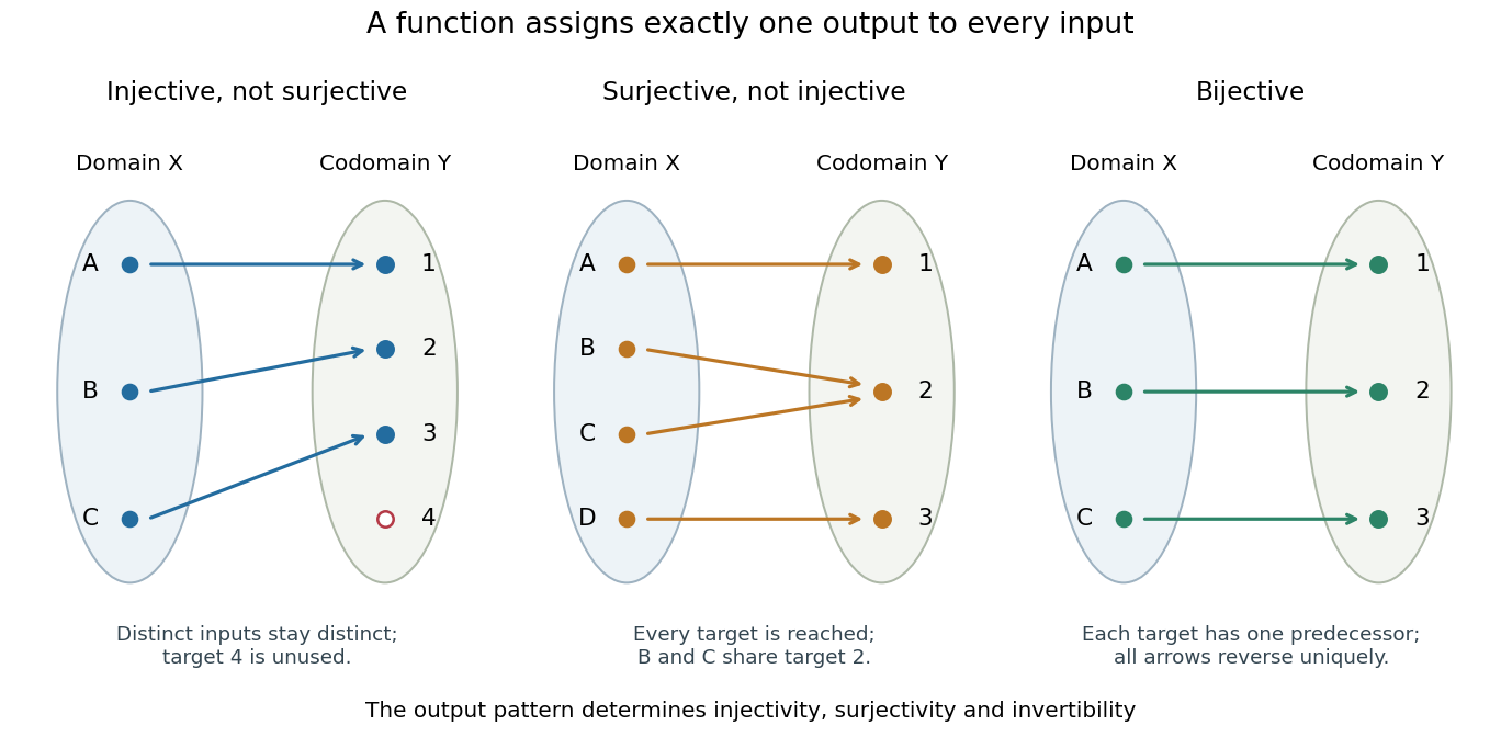
The chosen codomain matters even when the formula does not change. The function from to is not surjective, whereas the same rule from to is surjective. Both fail injectivity. Further restricting the domain of a function to makes it a bijection onto , with square root as its inverse function.
Functions make transformations composable: if and , their function composition is . Identifying each intermediate codomain prevents attempting to feed an output into a rule that is not defined there. When a transformation is a bijection, an inverse function recovers the original input without ambiguity. This is useful whenever information must be transported or a calculation reversed.
Function evaluation determines the function output for a specified function input in the domain of a function. Numerical integration uses these values at selected quadrature nodes.
A function input to a function is an element of its domain of a function , also called its argument. The corresponding function output is .
A function output is the value assigned by a function to a function input . It belongs to the codomain ; all such function outputs together form the image of a function .
For functions and taking values in the same field, their quotient of functions is defined by on the common domain of a function restricted to points where . Thus and on the real line give a quotient of functions defined only for .
The codomain of a function is its specified target set. The image of a function is a subset of the codomain, and equals it precisely for a surjective function. Changing a codomain can change whether the same input-output rule is surjective, as the quadratic function examples under function show.
A self-map is a function whose domain of a function and codomain are the same set. It need not be a bijection: a constant function on a two-element set is a self-map that merges its inputs. Self-maps can always be composed with one another, and all self-maps of a specified set form its full transformation monoid.
For functions and , their function composition is , defined by . The rightmost function is applied first. Matching the intermediate codomain and domain of a function makes the expression well-defined.
For self-maps of the real numbers, take and . Then , whereas . Thus function composition need not be commutative. It does have the associative property: both and evaluate to whenever each intermediate codomain matches the next domain of a function. The identity function leaves composition unchanged, making self-maps particularly useful as a monoid of transformations.
A germ at a point is an equivalence class of functions defined on a neighbourhood of the point: two representatives are equivalent if they agree on some smaller neighbourhood. A germ of a holomorphic function requires its representatives to be holomorphic functions; smooth and continuous germs use their corresponding classes of functions. The germ retains local behavior while forgetting the representative's values farther from the point.
A real-valued function is nonnegative when all its values are at least zero. Products and nonnegative linear combinations of nonnegative functions remain nonnegative. A nonnegative partition of unity gives convex combinations, hence a convex-hull bound for a geometric basis.
Two self-maps commute when . Induction then gives and for all nonnegative integers . Sharing a fixed point or invariant set does not by itself imply commutation. For rational sphere maps of degrees at least two, commutation does imply equality of their Fatou sets and Julia sets, by the commuting rational maps of degree at least two have the same Julia set theorem.
A finite modification agrees with the identity map outside a finite exceptional set. Sorting that set gives a unique finite record of pairs . Real-number pairing by separated digits encodes the record in , and placing length- records in disjoint intervals gives an injection from all finite modifications into the real line. Conversely, changing the value at one fixed point gives a real-parameter family, so the Cantor-Schröder-Bernstein theorem shows this family has continuum cardinality.
A pointwise periodic self-map returns each point to itself after a positive number of iterates which may depend on the point. It is a bijection: each finite cycle supplies predecessors; equality of two images can be undone by an iterate with an exponent one below a common multiple of the two periods. The set consequently decomposes into disjoint finite permutation cycles. Pointwise periodicity does not imply that one iterate is the identity on an infinite set.
A pointwise periodic self-map has a uniform positive period exactly when its finite cycle lengths are bounded. A uniform period is divisible by every length; conversely, bounded lengths divide the least common multiple of for some bound . Arbitrarily many bounded-length cycles are allowed. Every such map on a finite set has a uniform period. On any infinite set containing a countably infinite subset, cycles of unbounded finite lengths and fixed points elsewhere give a counterexample. Thus, with the usual axiom of choice assumption, the sets on which every pointwise periodic self-map has a uniform period are exactly finite sets.
A vector-valued function is a function with values in a vector space. For finite-dimensional real or complex target spaces, choosing a basis represents it by scalar coordinate functions; continuity and differentiability can then be checked coordinatewise.
A real-valued set function on an algebra of sets is finitely additive if it has the displayed property for disjoint pairs. It follows that . On a finite ambient set, induction gives , so arbitrary signed singleton weights describe all such functions. Summing the pointwise indicator function identity for the inclusion-exclusion principle against these weights proves the same formula for .
A real-valued set function is supermodular if it satisfies the displayed inequality. Its negative is a submodular set function. Equivalently, the gain from adding an element cannot decrease as the set grows. This is the defining property of a convex cooperative game, and makes coalition marginal allocations lie in the core of a cooperative game.
A set function is submodular if for every pair of subsets. Entropy submodularity is a fundamental example.
A function collision is a pair of distinct inputs with . An injective function has no collisions. For a two-to-one function every nonempty fiber has two elements and hence one unordered collision pair. Finding such a pair through an oracle is the task of quantum collision finding.
In the finite example under image and preimage of a function, the pair is a function collision: both inputs give zero. The function retains their shared output but loses the distinction between them. If a finite set has more inputs than the number of available outputs, the pigeonhole principle forces a function collision. Equal source and target cardinalities alone do not prevent one.
For a finite function, let be the cardinality of its fiber of a function over . The number of unordered function collisions is , because each pair must lie in one common fiber. The example's nonempty fiber sizes are , giving exactly one collision pair.
For a function and , its fiber of a function over is the set of all inputs producing that one output:Here is shorthand for a preimage of a singleton set, rather than a claim that an inverse function exists. A fiber can contain several inputs or be empty. It describes exactly which distinctions the function forgets.
For the finite function under image and preimage of a function, the fibers over are , , and the empty set, respectively. The nonempty fibers form a partition of a set: they are disjoint sets whose union is the domain of a function. Every input belongs to the fiber over its unique output, and two fibers with distinct output labels cannot share an input. A function is injective exactly when every fiber has at most one member; it is surjective exactly when every member of its specified codomain has a nonempty fiber.
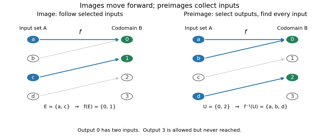
More generally, is the union of the fibers over all . The relation defined by is an equivalence relation, and its equivalence classes are precisely the nonempty fibers. The resulting quotient set is naturally in bijection with the image of a function. This links an input partition to the output values actually reached, without choosing one representative from each class.
Fibers are useful when an output is known but the input is not uniquely determined. A solution set is one fiber, and factorization through a surjection explains when another function depends only on the retained output. Quantum hidden subgroup problem algorithms use functions whose fibers are cosets, giving the same idea a structured form in group theory.
For a surjective function and a function , there is a unique function with if and only if is constant on each fiber of a function of . Define to be the common value on ; it is well-defined and unique because that fiber is nonempty. This uniquely specified value requires no simultaneous arbitrary choices.
For a concrete example, restrict the codomain of the finite function above to its image of a function , making surjective. Define , and . Then on gives : knowing the output of is enough to compute . If instead , no such can exist, because must be the same value.
The surjectivity assumption supplies uniqueness on the full target. If the original unused target value three were retained, the factorization would impose no condition on , and different extensions could agree on every actual input. Thus factorization through a surjection formalizes when a compressed description retains all information needed for a later calculation.
// Target: combinatorics.bigb
Translation shifts the argument without changing the shape of a function. On the real line, the displayed convention shifts a graph to the right by . Lebesgue measure invariance preserves every finite Lp norm; its Fourier transform is multiplied by .
For a function , its graph is the subset of . It differs from a graph in graph theory. A solution curve of a scalar differential equation can be a graph over its independent coordinate.
The map is continuous into the product topology. It maps a compact space onto the graph of a function of a continuous . Hence that graph is compact, whether or not the codomain is a Hausdorff space. Projection to is its continuous inverse.
For a continuous map with Hausdorff space , its graph of a function is closed in the product topology. If , choose disjoint neighborhoods of those two points in . Continuity supplies a neighborhood of whose image lies in the neighborhood of ; its product with the other neighborhood misses the graph.
A partial function from to assigns at most one value in to each element of ; it may be undefined outside a subset of .
A partial unary operation on a set is a partial function with specified domain and values in . A map preserving such operations must send each point of the source domain into the target domain and preserve its assigned value. It need not reflect whether the operation is defined.
Composition of partial functions is strict: is defined only if every is defined and is defined on the resulting tuple. An argument discarded by the outer function still has to be defined. A representation in a non-strict programming language therefore needs an explicit sequencing guard.
For a partial function , the domain is the subset . Outside this subset, evaluation of is undefined.
For a function and a subset , its restriction keeps the same values but allows only inputs in . Restricting the domain of a function can remove collisions and permit an inverse function, as the nonnegative quadratic function example shows. This changes the allowed inputs; it is different from keeping the inputs and changing the codomain.
A function class is a set whose elements are functions, usually sharing a common domain of a function and codomain.
The identity function on a set maps each to itself: . It changes no information. For every function , function composition satisfies and . The subscripts specify the appropriate source or target set. An inverse function reverses a bijection exactly when the two possible compositions are these identity functions.
An inverse function reverses a bijection. For , it is a function satisfyingEquivalently, for all and for all . We write . The superscript denotes reversal through function composition; it does not mean the pointwise multiplicative inverse . The preimage notation for a set is also distinct: a preimage exists even when no inverse function exists.
For a computed example, let be . Solving for gives . Thus and ; direct substitution gives and throughout the real line. In contrast, , which does not undo .
Why must be a bijection? If , applying gives , proving injectivity. For any , the equation supplies a source element, proving surjectivity. Conversely, a bijection supplies exactly one predecessor for each , defining a unique inverse function. A left inverse or right inverse requires only one of the two composition identities.
For on the real line, the equation has two solutions, , so its arrows cannot be reversed as one function on all inputs. The restriction to removes that ambiguity. As a bijection from onto , it has inverse function . The identity explains why works on the restricted domain of a function but fails for negative . [ref]
https://openstax.org/books/calculus-volume-1/pages/1-4-inverse-functions. OpenStax, inverse functions and domain restrictions
.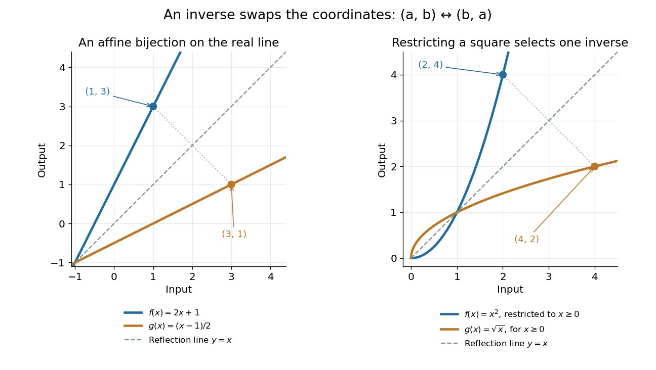
An inverse function swaps the input and output coordinates
. Left: the function graphs of and its inverse function are reflections across the line ; the points and correspond. Right: the nonnegative restriction and the square root have the same reflection relation. Their displayed portions lie in the first quadrant or on its boundary. Details.More generally, lies on the graph of a function precisely when lies on the graph of a function of its inverse function. This coordinate swap explains the geometric reflection and the horizontal line test. It also explains why inverse sensitivity is reciprocal locally: the inverse function rule divides by the original derivative at the corresponding input, when that derivative is nonzero.
For a real-valued function drawn in the plane, the horizontal line test asks whether every horizontal line intersects its function graph at most once. This is exactly injectivity, since two intersections at the same height mean two inputs have the same output. A missing height is compatible with injectivity, so an inverse function is then defined on the image of a function; it is an inverse on the entire specified codomain only when surjectivity also holds.
Suppose is continuously differentiable near with . It has a local inverse function near , andThe chain rule applied to gives the formula. The nonzero derivative condition also ensures local invertibility; it does not assert a global inverse function on an arbitrary larger domain of a function. For at , the corresponding output is , and the square root's derivative there is . At , this division is unavailable: the nonnegative restriction still has a square root inverse, but its finite derivative at zero does not exist. [ref]
https://openstax.org/books/calculus-volume-1/pages/3-7-derivatives-of-inverse-functions. OpenStax, the inverse function rule and corresponding evaluation points
.A right inverse of a function is a function satisfying . It forces to be a surjective function. A surjective linear map onto a finite-dimensional vector space has a linear right inverse: lift a basis of the target and extend by linearity.
The assertion that every surjective function has a right inverse is equivalent to the axiom of choice. Choice selects one member of each nonempty fiber of a function, giving a right inverse. Conversely, for a family of nonempty sets, the projection from the disjoint union onto is surjective. A right inverse selects one element from each , giving a choice function.
A left inverse of a function is a function satisfying . It forces to be injective, since equal images can be mapped back to equal original elements.
A projection is a function that fixes the points in its image: applying it twice has the same effect as applying it once. A coordinate projection can be represented this way when its target is identified with a retract; a linear projection additionally respects the vector-space operations.
For a coordinate projection map onto , write for the other factor. The map is surjective exactly when is empty or is nonempty. It is injective exactly when is empty or has at most one element. In particular, a surjection onto an empty Cartesian product need not induce a surjection onto a nonempty factor.
Functions and are conjugate through a bijection when . The bijection transports orbits and fixed points of every iterate of to the corresponding objects for .
A piecewise-linear function is linear on each member of a finite or locally finite partition of its domain into intervals or polyhedral pieces.
Between two prescribed values, linear interpolation assigns at , for . Joining successive samples produces a piecewise linear function. For a continuous function on a compact interval, interpolants along grids with mesh tending to zero converge in the uniform norm; their error is bounded by the modulus of continuity at the mesh size.
A real- or complex-valued function is bounded when the moduli of all its values have one finite upper bound.
An unbounded function has no finite bound on the moduli of its values.
On a nonempty domain of a function , a constant function has one fixed value in its codomain:For example, on the real line is a horizontal graph. Its image of a function is the singleton even though its domain of a function has infinitely many inputs. A constant function from the real line to the real numbers has derivative zero and every nonzero real period of a function; there is no smallest positive period. It supplies a reference level from which variation can be measured.
A constant map between vector spaces is a linear map only when its value is the zero vector, since a linear map must preserve zero. A nonzero constant map is still an affine map. In a Fourier series, the constant term records the period average, while the other terms describe oscillation around that level.
A function is nonconstant when two inputs in its domain of a function have different outputs. For example, on the real line is nonconstant, whereas the same rule restricted to is a constant function.
A global maximum is one type of extremum of a real-valued function; global minima reverse the inequality.
The negative part of a real-valued function is the nonnegative function . It records the magnitude of the negative values, rather than retaining their sign: if , then . Together with the positive part, it gives and . This decomposition defines the Lebesgue integral of a signed function and makes the integrability condition explicit.
A bijection is a function that is both injective and surjective: each element of its codomain is the output of exactly one element of its domain of a function. The two requirements exclude unused targets and merged inputs respectively. The finite example , , is a bijection from to , whereas adding an unused target makes that same rule fail surjectivity.
A bijection gives an inverse function by reversing every pairing. Conversely, a two-sided inverse function implies a bijection, as the proof under inverse function shows. This is useful for transporting structures without losing or identifying elements. It also defines equality of cardinality: two sets have equal cardinality exactly when a bijection pairs them. An infinite example is from the integers to the even integers, with inverse on that specified codomain. A proper subset can therefore have the same cardinality as an infinite set. [ref]
https://discrete.openmathbooks.org/preview/sec_intro-functions.html. Levin, functions: injections, surjections and bijections
.A periodic function repeats exactly after a nonzero shift of its input. For , a positive period of a function satisfiesOne interval of length therefore determines the whole function. For another domain of a function , a period must also preserve the domain, ; equality only where two domains happen to overlap is weaker. Periodicity is an exact translation of a function symmetry, rather than merely two similar-looking pieces of its graph.
The sine has fundamental period one. The function repeats after half a unit: the sine changes sign under that shift, but squaring removes the sign. The mixed function again has fundamental period one. All positive integer multiples of a period are periods, so specifying one period need not identify the shortest repetition.
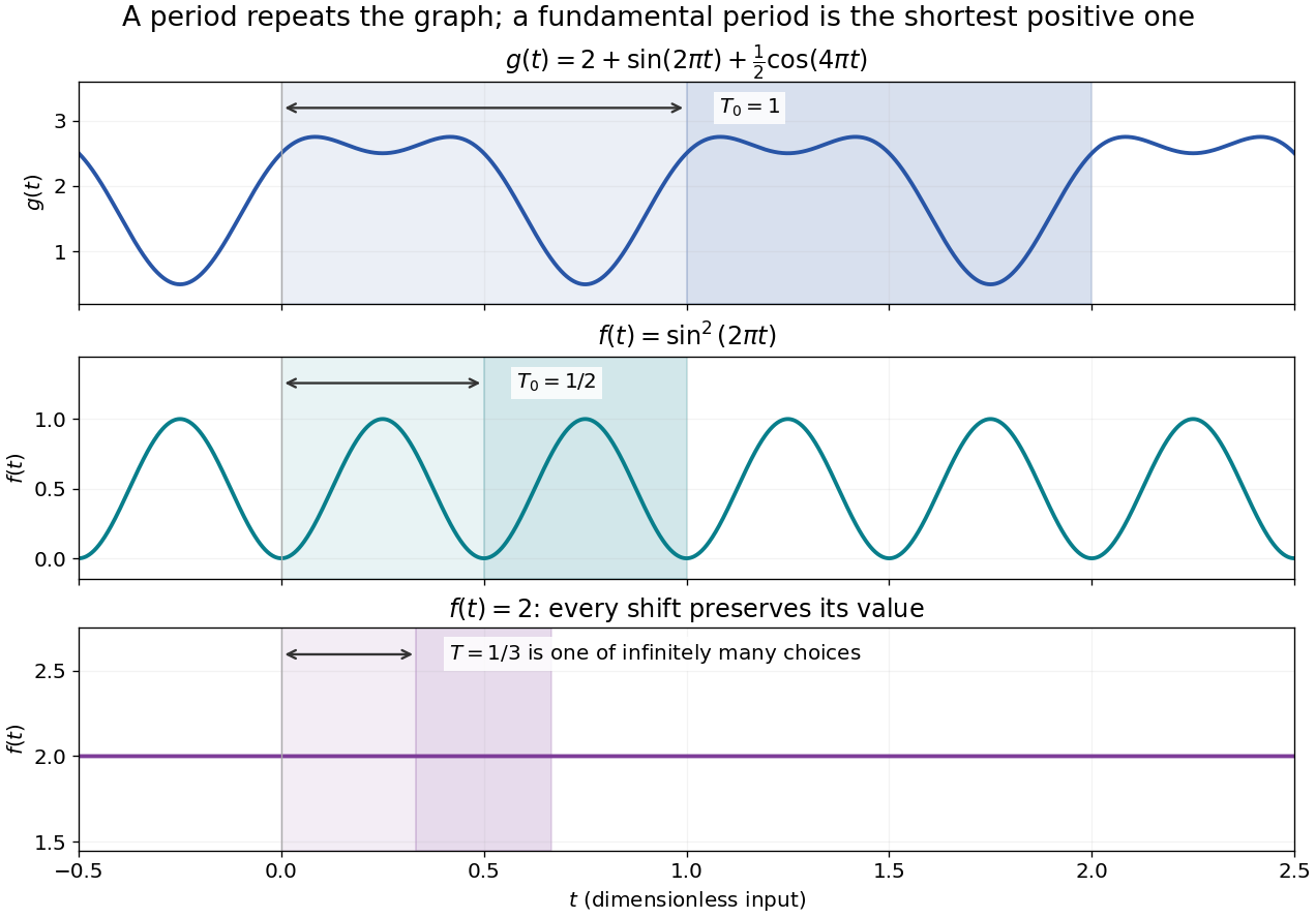
If the input is time and is the fundamental period, the frequency is and the angular frequency is . Repetition lets a Fourier series describe a cycle using sines and cosines; the period average separates the reference level from the oscillating terms. Strang develops this representation and its Fourier coefficients in §4.1 of Computational Science and Engineering by Gilbert Strang.[ref]
Fourier Series for Periodic Functions. §4.1; pp. 317
This connection grew out of a physical problem. In his 1822 book Théorie analytique de la chaleur by Joseph Fourier, Joseph Fourier used periodic functions to extend profiles beyond their initial interval while treating heat conduction. Chapter III, §§233–234 combines even functions and odd functions into sine–cosine expansions and rescales their period.[ref] A modern Fourier series interpretation still requires the appropriate convergence conditions.
A constant function has every real shift as a period and no fundamental period. Without continuity, even a nonconstant periodic function can lack a smallest positive period; periodic function without a least positive period gives a concrete example. The period group of a function organizes all these possibilities.
The fundamental period is the least positive period of a function, when one exists. For it is one; for it is . A periodic function need not have a fundamental period: a constant function has every positive period, and periodic function without a least positive period is a nonconstant exception. Every nonconstant real-valued function that is continuous and periodic on the real line does have a least positive period.
For a real-valued continuous function, the period group of a function is a closed subgroup: if periods tend to , continuity passes to the limit. If positive periods could tend to zero, integer multiples of those periods would approach any prescribed displacement , forcing . A nonconstant function therefore has a positive lower bound for its positive periods. Their infimum is itself a period by closedness. Subtracting an integer multiple of from any other period leaves a period in , which must be zero. This proves the stated structure without assuming differentiability.
Define the indicator function of the rational numbers on the real line by for rational and otherwise. Every rational shift preserves rationality and irrationality, so every nonzero rational number is a period of a function. Conversely, an irrational shift sends from value one to value zero, so it is not a period. The period group of a function is exactly , and the positive periods approach zero without a smallest one. The function is nonconstant and discontinuous everywhere; this is why continuity matters in continuous periodic functions have a least positive period.
Include zero when forming this set, even though a period of a function is normally required to be nonzero. For , is a subgroup of the additive group of the real numbers: composing two preserving shifts adds them, and reversing a preserving shift negates it. A constant function has period group . A nonconstant continuous real-valued function that is periodic has period group , where is its fundamental period.
A nonconstant meromorphic function on the complex plane is simply periodic when its group of periods is generated by one nonzero complex number. It is distinct from a doubly periodic elliptic function, whose period lattice has two real-linearly independent generators. Single periodicity alone imposes no algebraic addition law.
For fixed positive integer period , integer-valued periodic functions on are in bijection with and hence form a countable set. Their union over periods is a countable union of countable sets. In contrast, period-one integer-valued functions on can prescribe arbitrary binary values on its infinitely many distinct classes modulo . The power set of a countably infinite set injects into them, proving uncountability.
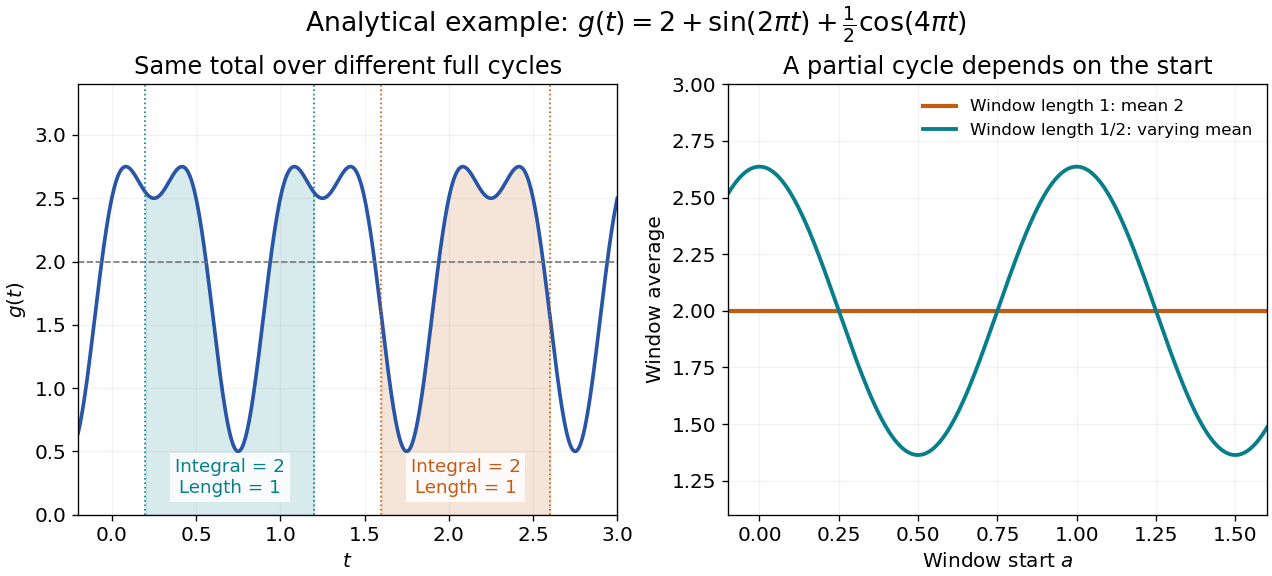
The period average extracts the reference level of an integrable function that repeats. For a real- or complex-valued periodic function with positive period of a function , assume is Lebesgue integrable on every bounded interval. Its average isThe answer is independent of the starting point . Splitting a shifted interval at the old endpoint and using moves its extra piece back into the missing piece. The interval length must be a period; an arbitrary window can give a different average.
For , every length-one window has average : both oscillating integrals vanish over that window. A half-unit window instead has average , which depends on its start. Thus a short sample of an oscillation can bias an estimate of its reference level even when the full-cycle average is known exactly.


In the complex Fourier series convention with basis , the zero-frequency Fourier coefficient is . This assertion defines the coefficient even when an additional convergence theorem is needed to reconstruct from its series. Strang's §4.1 explicitly identifies that constant coefficient with the average.[ref]
Fourier Series for Periodic Functions. §4.1; pp. 317
Averaging a square measures something different from averaging its original function. For the illustrated , orthogonality of the trigonometric terms gives , whereas . Its root mean square is therefore . Similarly, the period average of is . A zero mean need not imply a zero mean square.
A triangular wave is a continuous piecewise linear periodic function whose slope alternates between two values. The even -periodic extension of from is for . Its Fourier cosine series contains a constant term and odd modes with coefficients proportional to the inverse square of the mode number. Such extensions describe reflection under Neumann boundary conditions.
Articles by others on the same topic
There are currently no matching articles.