
The log-likelihood is the natural logarithm of the likelihood function:For positive finite likelihood, the natural logarithm is a strictly increasing function, so the maximizing parameter values are unchanged. Set where ; the same ordering then includes zero-likelihood boundaries whenever a positive finite maximum exists. For independent and identically distributed random variables, a product becomes a sum,This makes derivatives simpler and avoids forming products of tiny numbers in floating-point arithmetic. These equal-maximizer and additive formulas underlie the worked calculations in MIT 18.05, Reading 10b, section 3.1.
For the ordered sample of eight successes and two failures in likelihood function, on ,The score equation gives , hence . The negative second derivative proves strict concavity, so this is the unique interior maximum. Both counts are positive, so , while inside: the same point is the unique global maximum on . Counting only successes adds to the log-likelihood, leaving both derivatives and the MLE unchanged. For all-success or all-failure samples, the boundary analysis in maximum-likelihood estimator applies instead of an interior score equation.
The two panels below compare successes out of ten Bernoulli trials. Their peaks are at . The left panel uses relative height; the right panel uses the log-likelihood difference from each peak. These are the same comparison on two scales:A difference of means relative height , and a difference of means ; the log-likelihood scale makes small relative heights easier to see. Neither vertical axis is a parameter probability density function. The zero likelihood endpoints have log-likelihood and are outside the finite vertical range in the right panel.
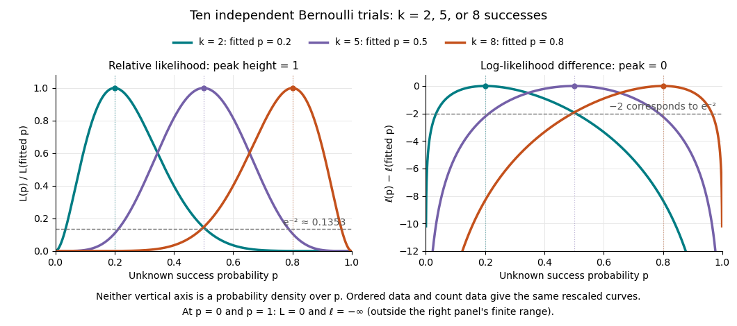
Ten Bernoulli trials: relative likelihood heights and log-likelihood differences share the same peaks
. Details. 
Multiplying a likelihood function by a positive parameter-independent constant adds a constant to its log-likelihood. Subtracting its peak removes that constant. This is why the ordered-data and count-data curves coincide in this figure after rescaling. When differentiable, the gradient of the log-likelihood is the score function; the negative Hessian matrix is the observed information. A solution of a score equation still needs checking against other stationary points and boundaries: maximizing the log-likelihood does not automatically make it concave.
New to topics? Read the docs here!