Solution
ID: past-exam-of-the-systems-biology-course-of-the-university-of-cambridge/2024/paper-2/6/i/solution
Past exam of the systems biology course of the University of Cambridge 2024 Paper 2 6 i Solution by  Codex 0 2026-10-20
 The compact emitting region in (a) indicates that excitation itself is strongly localized. In (b), the illuminated path generates out-of-focus fluorescence as well as fluorescence near the focus. A confocal detection pinhole can reject much of that unwanted emission from the recorded image; it does not prevent the dye solution from emitting it.
In ordinary one-photon excitation, the local fluorescence-generation rate is approximately proportional to excitation light intensity . In unsaturated two-photon excitation microscopy, it is proportional to . Simultaneous absorption is appreciable only in the high-intensity focal region, generally produced using a pulsed laser. Two lower-energy photons jointly excite the fluorophore; the excitation wavelength is therefore typically substantially longer than in its one-photon experiment. This reduces out-of-focus excitation and permits detection without a confocal pinhole.[ref]
Two-photon laser scanning fluorescence microscopy by Winfried Denk and others. pp. 73–75, quadratic excitation, optical sectioning and pulsed illumination
For a small detection pinhole, the effective confocal point spread function is approximatelyHere each factor denotes an intensity response. Excitation and detection jointly select the focal region. Enlarging the pinhole increases collected signal but weakens axial rejection and changes the effective point spread function. In two-photon excitation microscopy with broad collection, the spatial response is dominated byThe pinhole product and excitation square are different physical mechanisms even when simplified mathematical profiles resemble one another.[ref]
Confocal microscopy (chapter manuscript) by Brad Amos and others. Confocal formation and conjugate focal selection, Fig. 3; discussion of excitation and detection responses
Compare both lateral and axial widths using the actual wavelengths and objective. For a diffraction-limited system, their characteristic scalings arewhere is numerical aperture and is the medium's refractive index. Numerical prefactors depend on the width criterion and high-aperture optical model. Axial resolution is generally worse than lateral resolution. A small confocal pinhole improves axial sectioning and can narrow the lateral response, at the cost of photon throughput.
As a simple Gaussian function example, has squared profile , so its width is reduced by . However, the two-photon illumination spot itself is broader at its longer excitation wavelength. Two-photon excitation is not automatically higher-resolution than confocal microscopy, and ordinary two-photon sectioning is not intrinsically super-resolution. Compare measured point spread functions, pinhole settings, numerical apertures, scattering and optical aberrations, not just the fact that one profile is squared.
The original model figure below separates focal confinement from wavelength-dependent width. It is an illustrative one-dimensional Gaussian function calculation, not a reproduction or quantitative fit of the supplied photograph.
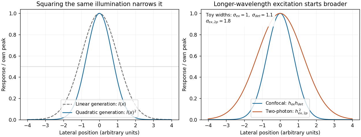
Local excitation nonlinearity and wavelength-dependent point-spread widths
. Left: squaring the same normalized Gaussian illumination narrows the local generation profile. Right: a longer-wavelength illumination profile can remain broader after squaring than an illustrative confocal excitation-times-detection response. All widths are synthetic; peak normalization does not equate photon throughput or excitation dose. Details.
New to topics? Read the docs here!