A laser generates amplified light through stimulated emission. Its name abbreviates “light amplification by stimulated emission of radiation”. Lasers supply the intense beams used in optical tweezers; optical coherence also makes them useful for wave interference measurements. [ref].
In the usual material picture, a gain medium stores energy supplied by pumping, for example by incident light or an electric current. Stimulated emission transfers that stored energy to a selected optical normal mode, while competing photon absorption removes light. Producing net optical gain requires a suitable population distribution, such as population inversion in the simple model below.
A familiar laser oscillator uses mirrors to return light through the gain medium. This optical feedback favours resonant normal modes; a partly transmitting mirror lets useful power escape. Feedback and mode selection have different implementations, including ring arrangements: every laser need not resemble the same two-mirror device. The laser threshold example treats just that device. [ref]
https://ocw.mit.edu/courses/res-6-006-video-demonstrations-in-lasers-and-optics-spring-2008/37b4c2aa5a6e3e0c119688024ce90ce5_Iqp7NxnwaGY.pdf. Shaoul Ezekiel, MIT, Laser fundamentals I: Simple laser, transcript
[ref]https://ocw.mit.edu/courses/6-974-fundamentals-of-photonics-quantum-electronics-spring-2006/18f30fad63a62ef4dd894d3752b55a60_chapter7.pdf. Franz Kärtner, MIT 6.974, Chapter 7, §7.1: laser oscillator concept
.The useful combination is concentrated power and controlled optical normal modes. It gives optical tweezers a localized source of force and wave interference measurements a source with useful optical coherence. A laser can nevertheless emit several frequencies; “laser” alone does not guarantee a single frequency. [ref].
An original experimental landmark is T. H. Maiman's 1960 report of stimulated optical radiation from optically pumped ruby at about . His paper describes both the pumping path and the observed emission, connecting stored material energy with amplified light. [ref]
Stimulated Optical Radiation in Ruby by Theodore Harold Maiman. T. H. Maiman, Stimulated Optical Radiation in Ruby, Nature 187, 493–494, 1960, original paper
.Sustained stimulated optical emission in a resonator mode, supplied by the pump and reinforced through optical feedback. Its onset is governed by the laser threshold; an amplifying single pass alone does not establish oscillation.
The transition between the upper and lower working energy levels that supplies stimulated laser emission. It is one part of the pumping cycle, distinct from the complete laser device and from an auxiliary pump transition.
A pumping scheme with an auxiliary pump level, an upper laser level, a rapidly emptied lower laser level and a ground reservoir. Efficient lower-level removal reduces the population cost of inversion compared with a ground-state-terminated three-level laser, while cavity loss still imposes a finite laser threshold.
The material in which pumping produces optical gain through stimulated emission. Its inversion density, mode-overlap volume and emission cross section determine whether the gain overcomes cavity losses.
A laser rate equation approximates coupled evolution of population inversion and intracavity photon number, including pumping, spontaneous emission, stimulated emission and optical cavity losses. A simple model is , , where compatible normalizations absorb mode-volume factors. Large excess optical gain drives rapid field growth until inversion depletion reduces it below threshold.
If a fraction of an otherwise uniform optical cavity contains gain medium, define upper-state density per gain volume but photon density per whole cavity volume. Stimulated upper-state depletion is , while cavity photon production is . Thus and . Above threshold and , where .
Small perturbations of a class-B laser exchange excitation between the upper-state population and cavity photon number. Linearization about a four-level lasing state gives . Its damped oscillation frequency is . Long population lifetime compared with photon lifetime permits underdamped relaxation.
Large startup excursions of a laser can accumulate population above threshold and then release it through a short stimulated-emission pulse. Inversion depletion and pump recovery can produce a damped sequence of spikes. This is a nonlinear transient, distinguished from small-signal laser relaxation oscillations and from externally imposed Q-switching.
Q-switching creates a short high-energy optical pulse by first storing population inversion while an optical cavity has high loss, then increasing its quality factor so that stimulated emission rapidly extracts the stored excitation. Its duration depends on photon lifetime, excess optical gain, inversion depletion and switching time; it is not fixed by a universal time-bandwidth equality.
For an ideal pulse with negligible stored seed photons and useful output accounting for all cavity photon loss, the extracted energy is . The factor converts inversion depletion into stimulated transitions. With over-pumping , the nonzero extraction branch satisfies . A fraction of the maximum energy requires .
A laser based on an excited molecular species. ArF systems commonly provide 193 nm radiation for projection lithography.
In laser ablation, concentrated optical energy removes or disrupts material locally. Cutting a loaded cellular structure and observing recoil can probe its mechanics, but the recoil also depends on dissipation and surrounding constraints.
For a vertical optical transition between parabolic energy bands with common carrier temperature, net stimulated emission has occupation factor . The monotonic Fermi-Dirac distribution makes this positive exactly when the quasi-Fermi-level splitting exceeds the transition photon energy. An allowed transition must also lie above the band gap. Broadening, band degeneracy and a zero-temperature occupation window require their own qualifications; this condition alone does not establish laser threshold.
A laser whose gain medium contains dye molecules. Its tunable wavelength permits laser spectroscopy of different spectral lines.
A three-level laser pumps emitters out of their ground state into a higher pump state, which rapidly relaxes into the upper lasing state. The lower lasing state is the ground state itself. Photon absorption on the lasing transition therefore competes with stimulated emission until enough emitters have been removed from the ground state. This is the ground state depletion problem implicit in population inversion.
The model below treats nondegenerate lasing energy levels with equal absorption and emission cross-sections. Its inversion condition is . Real materials require the relevant sublevel populations, degeneracies and transition strengths; the simple half-population condition should not be imposed on every optical transition. Extra levels let the pump and the emitted light act on different transitions, avoiding the steady two-level saturation limit discussed in population inversion.
In a three-level laser whose lower lasing level is the ground state, fast relaxation from a pumped higher level feeds a long-lived upper lasing level. With equal lasing-level degeneracies, negligible pump-level population and pump rate R per ground-state emitter, the no-light stationary rate equation gives . Positive population inversion therefore requires more than half the active emitters to leave the ground state. This is a transparency threshold; optical resonator loss imposes an additional positive-gain requirement. Degenerate sublevels require population comparisons weighted by their statistical weights and transition strengths.
A ruby laser uses chromium ions in ruby as its amplifying medium. Maiman's report identifies a metastable state fed by optical excitation and red emission near .[ref]
Stimulated Optical Radiation in Ruby by Theodore Harold Maiman. Stimulated Optical Radiation in Ruby, opening and level-scheme paragraphs
The pump stores excitation in the medium; stimulated emission transfers it into the optical field. The simplified three-level laser rate equation explains why the stored population and the output pulse evolve together.Theodore Harold Maiman and Irnee J. D'Haenens obtained laser action in May 1960. Their arrangement put a ruby rod inside a helical xenon flashlamp. Increasing excitation produced a marked intensity threshold, with subsequent measurements showing narrowing of the ruby emission line.[ref]
Theodore Harold Maiman by Irnee J. D'Haenens. Participant recollection: apparatus opening; paragraphs beginning In early 1960 and Subsequent measurements
The 1960 letter describes silvered parallel crystal faces and compares low- and high-excitation spectra.[ref]Stimulated Optical Radiation in Ruby by Theodore Harold Maiman. Apparatus paragraph and Fig. 2, low- and high-power spectra
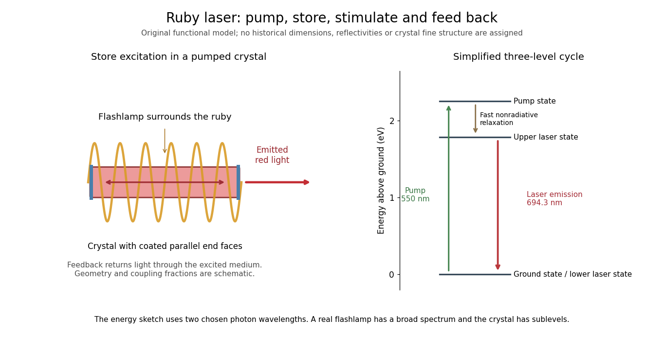
The controls answer different questions. Increased brightness establishes neither optical feedback nor narrow-band emission by itself: ordinary fluorescence can also brighten with pumping. Comparing spectra at lower and higher excitation, retaining the same optical collection geometry, tests a change in the emission process. Spectrometer resolution, response saturation and heating can alter an apparent line profile; a bright spot alone cannot distinguish those effects. These are interpretation requirements, rather than additional measurements attributed to the short original letter.
Several experimental models were made. The Smithsonian's surviving head has uncertain priority, and its installed crystal came from a later experiment.[ref]
Head Piece from Maiman Laser by Smithsonian Institution. Description: multiple experimental models, uncertain first-unit identification and replacement crystal
The functional diagram therefore describes the optical mechanism rather than claiming to reconstruct the first surviving unit.Consider an original reduced model with a fixed number of active emitters. Let be the upper lasing-state fraction, the ground-state fraction, and the number of cavity photons per emitter. Assume the pump state empties rapidly, so its population can be neglected. Measure time by , where is the upper state's spontaneous lifetime. Let be the effective pump rate, the dimensionless stimulated-coupling coefficient, the photon-loss rate in these units, and the fraction of spontaneous decays feeding this optical normal mode. The rate equations areEach term has a physical role. Pumping transfers emitters out of the ground state; spontaneous emission removes upper-state population. The net stimulated term includes emission from fraction and absorption by fraction , giving their difference . A stimulated transition removes one stored excitation and creates one cavity photon, or does the reverse. The factor accounts for spontaneous emission into the selected mode without pretending that all spontaneous emission enters it.
For negligible cavity light, the upper-state equation is linear. A constant pump applied to givesThus this model first permits population inversion at . Positive optical gain is still insufficient for an oscillator: the gain must exceed the complete laser threshold, including photon loss. The small-signal photon growth coefficient changes sign whenIf , even complete inversion cannot exceed the assumed loss in this model. For chosen and , the threshold population is and the pump threshold is . At , the unsaturated population first reaches at . These numbers are stipulated examples, not ruby material parameters.
In the steady limit with nonzero cavity light and negligible spontaneous seeding, the photon equation requires . The upper-state fraction is therefore fixed near while increased pumping principally increases the photon population. Substituting into the population equation givesFor , and , this predicts and . The inversion does not rise indefinitely above threshold. A finite supplies seed photons and smooths the ideal onset; with and exactly , the deterministic equations remain on the zero-photon solution even when that solution is unstable. This distinguishes instability of an unseeded state from actual startup of a noisy optical field.
A short optical pulse can draw on previously stored excitation. In the original calculation below, , , , , and for , followed by . The cavity field initially remains small while pumping fills the upper state. Once sufficient gain develops, the photon population grows and depletes the stored inversion. Continuing pump action can refill it, giving relaxation oscillations in this simple model. This is not a fit to Maiman's recorded output.
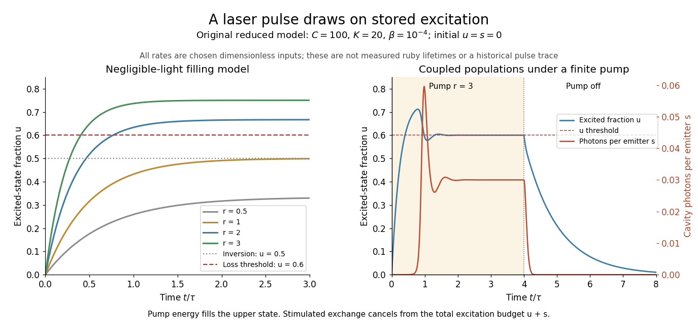
Ground-state depletion delays startup, and cavity light then drains stored excitation
. Original three-level laser rate equation calculations. Left: negligible-light upper-state fractions for several constant pumps, compared with the chosen . Right: coupled upper-state and cavity-photon populations for , , and a pump of switched off at . The rates and times are dimensionless teaching inputs, not measured ruby lifetimes or a historical pulse trace. Details.The equations expose the excitation budget underlying conservation of energy. Adding them cancels the stimulated exchange:Pumping supplies excitations; nonlasing decay and cavity loss remove them. Integrating gives the boundOnly part of the cavity loss may be useful output; passive absorption is also a loss. The pulse's instantaneous power can draw on stored excitation, while its total extracted energy still obeys the integrated budget. The model also preserves and : at each boundary its derivatives point inward or along the boundary.
There is a further energy cost in the pump cycle. For one absorbed pump photon producing at most one emitted laser photon, the ideal energy-conversion bound isChosen wavelengths and give about before other losses. The missing energy can leave through nonradiative relaxation and heating. Actual efficiency also depends on how much pump light is absorbed, unwanted decays and optical losses; a population model alone cannot predict it.
Laser detuning is the difference between a laser angular frequency and a specified atomic resonance angular frequency. Red detuning has ; blue detuning has . The sign matters in laser cooling: a moving atom can see a red-detuned laser closer to resonance because of the Doppler effect.
Stimulated emission is emission induced by incident light, in contrast with the unprompted decay in spontaneous emission. It supplies the amplification mechanism of a laser. [ref].
For an emitter with upper and lower energy values , the resonant photon has frequency satisfyingwhere is the Planck constant. In the elementary photon picture, an incident photon stimulates an emitter in the upper quantum state to emit an additional photon into the same optical normal mode, with the same frequency, propagation direction and photon polarization. The emitter supplies the extra energy; the stimulating photon is not consumed. This builds the existing field and its optical coherence. An emitter in the lower quantum state can instead undergo photon absorption, so stimulated emission alone does not establish net optical gain.
For example, a gap corresponds to and a vacuum wavelength of about . One ideal stimulated emission event converts one incoming photon into two outgoing photons in the selected optical normal mode, adding of light energy while lowering the emitter's energy by that amount.
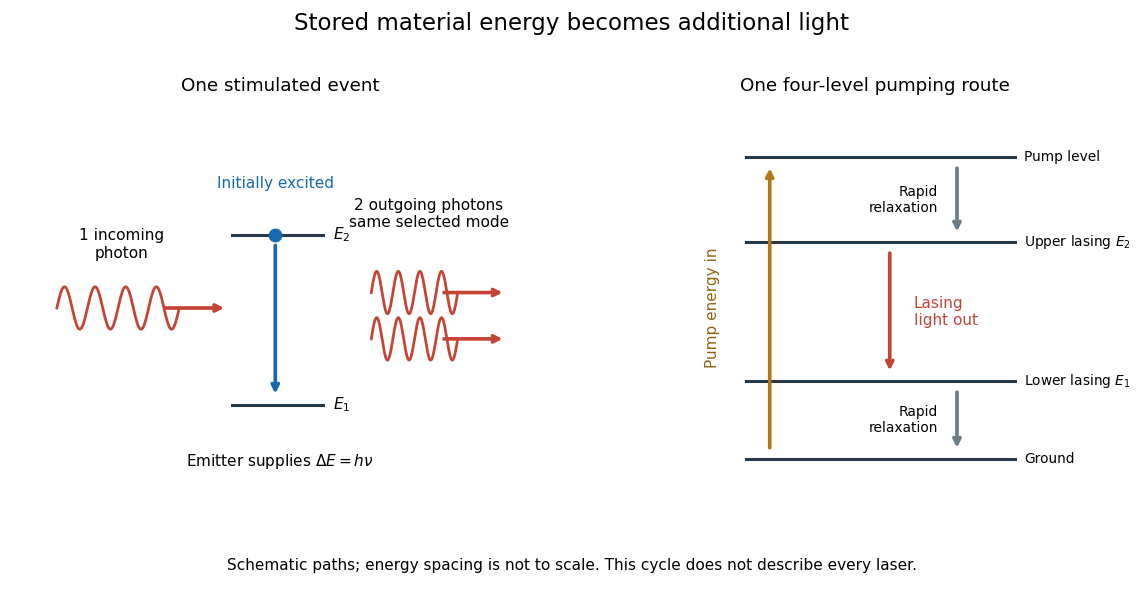
Stimulated emission and one illustrative four-level laser pumping cycle
. Left: one incoming photon induces an additional photon while the emitter falls from to . Right: pumping supplies energy, rapid relaxation feeds the upper lasing state, stimulated emission supplies light, and rapid lower-state relaxation completes a four-level cycle. These paths are schematic, not universal to all lasers; line spacing is not to scale. Details.The effective area converting incident photon flux into a stimulated emission rate for a specified transition, frequency, polarization and sublevel distribution. For statistically populated energy levels of statistical weights , the Einstein coefficients imply . The related absorption cross section therefore differs when the statistical weights differ.
The creation-operator matrix element makes emission into a radiation mode proportional to . The part is stimulated emission and the remaining part is spontaneous emission. Absorption has the corresponding occupation factor .
A population inversion puts more emitters in the upper than in the lower quantum state of a transition in the nondegenerate two-level model. Let be their number densities. Equal stimulated-transition strengths make the emission rate proportional to and the competing photon absorption rate proportional to , so net optical gain is proportional to . For and , the difference is positive; swapping them makes the medium absorb. Equal populations give zero net stimulated contribution. With degenerate levels, the relevant comparison uses populations per statistical weight of an atomic level, rather than simply .
Why pump through extra levels? Ordinary steady resonant pumping of a nondegenerate two-level system drives both photon absorption and stimulated emission. With equal induced rate and upper-state decay rate , its elementary population equation isat a stationary population. Increasing this pump saturates towards ; it cannot sustain population inversion in this model. This is a steady rate-equation conclusion, not a universal prohibition on all driven two-level dynamics or all possible laser gain mechanisms. [ref]
https://ocw.mit.edu/courses/6-974-fundamentals-of-photonics-quantum-electronics-spring-2006/2641db6431ea70989c29e8512d5d91a7_chapter6.pdf. Franz Kärtner, MIT 6.974, Chapter 6, §§6.7–6.8: saturation and rate equations
.In a familiar three-level path, pumping excites a higher level which relaxes into the upper lasing level; the lower lasing level is the ground state, so substantial ground-state depletion is needed. A four-level path also provides rapid emptying of the lower lasing level into a separate ground state. Suitable lifetimes then allow accumulation above and depletion below the lasing transition. Pumping still supplies the energy: extra levels provide a route to population inversion, not free energy. [ref]
https://ocw.mit.edu/courses/6-974-fundamentals-of-photonics-quantum-electronics-spring-2006/18f30fad63a62ef4dd894d3752b55a60_chapter7.pdf. Franz Kärtner, MIT 6.974, §7.2.1: three- and four-level laser media
.A pump feeds an auxiliary high level, rapid relaxation populates the upper laser level, and rapid decay empties the lower laser level. This separates pumping from the laser transition and helps sustain net stimulated gain. Gain saturation and cavity loss still determine the oscillating steady state.
Optical gain is amplification of light by a medium. Here the small-signal intensity gain coefficient has units : for fixed populations, a weak beam obeysin the nondegenerate resonant two-level model, with common transition cross-section . Thus includes the competition between stimulated emission and photon absorption on that transition. Separate passive intensity loss gives . Both coefficients describe light intensity, not wave amplitude; the corresponding field-amplitude exponent is half as large. [ref]
https://ocw.mit.edu/courses/6-974-fundamentals-of-photonics-quantum-electronics-spring-2006/2641db6431ea70989c29e8512d5d91a7_chapter6.pdf. Franz Kärtner, MIT 6.974, §§6.7–6.8: amplification and stimulated-transition cross-section
.For , and , the single-pass intensity multiplier is . This is amplification during one passage, before mirror losses. Population inversion can therefore yield positive optical gain while the complete oscillator remains below laser threshold.
A medium in which stimulated emission can increase an incident optical signal. Its unsaturated gain, saturation response and loss budget determine the propagation. A population balance with negative net gain instead describes absorption.
An open pumped two-level system amplifier with fixed upper-state source , upper spontaneous emission only into the lower energy level, and lower-state removal rate . Let , and . Steady rate equations give and . Consequently the optical gain is with . Lower-state removal controls whether population inversion is possible, while its lifetime cancels from this model's saturation intensity. Different upper-state branching or a nonconstant pump generally changes that conclusion.
The frequency range over which an amplifying medium supplies appreciable optical gain. Its width must be stated with a gain-profile convention.
Narrowing of a pulse spectrum when the central frequencies receive larger optical gain than its wings. Phase correction alone cannot restore the suppressed spectrum.
In a simple two-mirror oscillator, laser threshold is the small-signal optical gain at which a resonant optical normal mode exactly replaces its round-trip intensity loss. Assume constant intensity coefficients and throughout a one-way distance , and mirror intensity reflectivities . One round trip has multiplierTwo traversals give the distance ; multiplying the two mirror factors completes the bookkeeping. Setting and taking a logarithm givesThe reflectivities here are intensity fractions, not field-amplitude reflectivities. A shorter gain region or nonuniform loss requires replacing the path exponent by the appropriate path integral. The balance also presumes a permitted resonant optical normal mode. [ref]
https://ocw.mit.edu/courses/6-974-fundamentals-of-photonics-quantum-electronics-spring-2006/18f30fad63a62ef4dd894d3752b55a60_chapter7.pdf. Franz Kärtner, MIT 6.974, §§7.1 and 7.5: round-trip balance and steady state; intensity convention specified here
.For , , and , the threshold is . At , : a small circulating signal decays even though the material has positive optical gain. At , : the signal initially grows. Raising passive loss or lowering mirror reflectivity raises laser threshold.
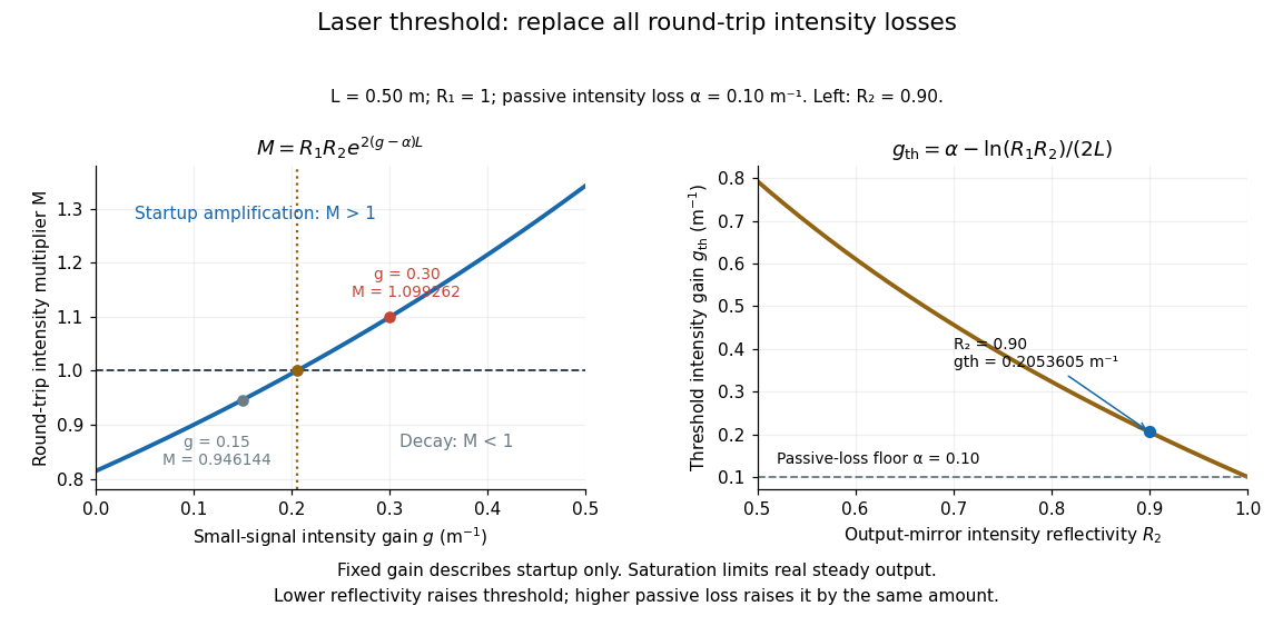
For , the fixed-gain recurrence predicts startup amplification, not infinite actual output. Growing light intensity depletes the available population inversion, reducing optical gain through saturation. In the simplest steady oscillator, the saturated round-trip gain balances loss and pumping supplies the outgoing power and dissipated energy. The small-signal model locates the onset; it does not determine the final output power. [ref]
https://ocw.mit.edu/courses/6-974-fundamentals-of-photonics-quantum-electronics-spring-2006/18f30fad63a62ef4dd894d3752b55a60_chapter7.pdf. Franz Kärtner, MIT 6.974, §7.5: gain saturation and steady output
.The pump power or pump rate at which an optical resonator's gain first compensates its round-trip loss. It depends on the population balance, mode overlap and loss budget; it is distinct from an unqualified value of the material gain coefficient.
If and are intensity gain and loss per length, a linear cavity has round-trip intensity multiplier . Threshold occurs when it equals one, giving . Phase resonance and the gain bandwidth determine which modes can oscillate.
An optical frequency comb has evenly spaced optical spectral lines, or teeth. A mode-locked laser supplies short optical pulses at repetition frequency , the tooth spacing. The carrier-envelope offset frequency positions the whole ruler:Only teeth within the emitted optical spectrum are present; the extrapolated intercept need not be an emitted tooth.[ref]
Passion for Precision by Theodor W. Hänsch. Passion for Precision, p.157: tooth relation
The achievement associated with John L. Hall and Theodor W. Hänsch is a practical bridge between optical frequencies and countable electronic frequencies. Instead of constructing a separate chain of lasers for each optical measurement, a broad comb supplies many linked reference teeth. Stable lasers, short optical pulses and strong nonlinear optics in optical fibers came together around 1999–2000.[ref]
Nobel Lecture: Defining and measuring optical frequencies by John L. Hall. Nobel Lecture: Defining and measuring optical frequencies, pp.1288–1291: chains and comb development
Mode locking fixes relative phases between longitudinal normal modes of a laser, allowing short optical pulses. The same optical spectrum with wandering relative phases would not supply that stable pulse train.[ref]
Passion for Precision by Theodor W. Hänsch. Passion for Precision, p.157: coupled modes
Here is an original finite-mode model, with the convention that a positive frequency has time dependence :These field coefficients follow a Gaussian function and have aligned phases at . Choose and write . Since for every integer ,The pulse light intensity repeats every although the field needs four periods to repeat. At the pulse centers, , , and . A detector of light intensity alone therefore cannot distinguish this offset from zero. This model has far fewer teeth than a practical optical comb; its normalized time and frequency scales are chosen to make the carrier oscillations visible.
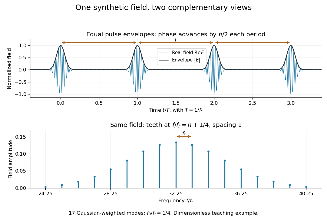
A short proof of the converse uses the Fourier series. If , then is periodic with period . Its Fourier series has frequencies ; restoring the removed factor shifts every tooth by . A finite observation time broadens the spectral peaks; it does not change this ideal infinite-train relation.
The circulating optical pulse itself changes the cavity response so that a short, intense waveform is favored. A saturable absorber reduces loss at high intensity; a semiconductor saturable-absorber mirror is one implementation. No external periodic timing drive is required, although stable operation still depends on gain and loss dynamics.
An external periodic modulation of cavity loss, gain or phase fixes the relative phases of its longitudinal cavity modes. A transmission window produced with an electro-optic modulator at the pulse repetition frequency selects a circulating optical pulse. Modulation bandwidth and dispersion constrain the attainable pulse duration.
The carrier-envelope offset frequency expresses the carrier's pulse-to-pulse phase slip relative to its envelope. Fixing the repetition frequency leaves this slip undetermined.[ref]
Defining and Measuring Optical Frequencies: The Optical Clock Opportunity – and More by John L. Hall. Defining and Measuring Optical Frequencies: The Optical Clock Opportunity – and More, p.131: offset
With the positive-exponential convention derived above, modulo . Changing translates every tooth equally; differentiating at fixed givesThus at , a chosen change in spacing moves that tooth by if stays fixed. The large multiplier is why a stable-looking pulse train is insufficient for accurate optical metrology.Comb self-referencing compares two parts of one optical frequency comb. Coherent broadening supplies an octave, a factor of two in frequency. Second-harmonic generation doubles a red tooth; a photodiode detects its beat with an original blue tooth.[ref]
Introduction to Self-reference Comb Laser by Comblaser Laboratory, Department of Physics, National Central University. Introduction to Self-reference Comb Laser, Fig.1 explanation
Applying the tooth formula givesThe doubled branch carries , while the original high-frequency branch carries : their difference retains exactly one offset.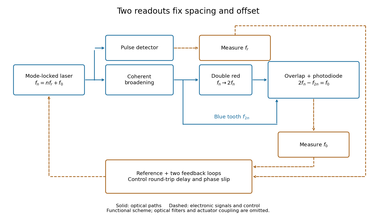
Read the tooth spacing and offset through separate electronic signals
. Original functional comb self-referencing scheme. Solid optical paths bring doubled red light and original blue light to one detector. Dashed electronic paths connect both readouts to a common reference and feedback controls. Actuators can affect both parameters. Details.The displayed difference uses the order doubled tooth minus original tooth. An ordinary electronic frequency counter returns a nonnegative beat magnitude; spectral selection and known electronic shifts must identify whether it represents , , or a shifted version. Coherent broadening, overlapping photon polarization, spatial alignment and temporal overlap are required. Merely producing a broad patch of colored light does not establish a usable offset signal.
The 2000 experiment prepared optical pulses with a mode-locked laser and broadened them in an air-silica microstructure optical fiber. A wavelength-selective beam splitter separated red and blue light. A nonlinear crystal doubled the red branch; the blue branch received a known acousto-optic shift. A filter selected recombined light for an avalanche photodiode, supplying an electronic beat. Mirror translation controlled repetition frequency; mirror tilt controlled offset with coupled effects. Separate delayed-pulse interference tested programmed phase changes. Alternative envelope fits and unmatched optical reflections were examined as checks and limitations.[ref]
These readouts answer different questions. The electronic beat closes a feedback loop; changing its setpoint and checking the delayed-pulse phase tests whether that control reaches the optical waveform. Neither readout alone establishes the accuracy of an unknown optical frequency. That additionally requires a calibrated time reference, the correct tooth number and beat sign, and checks for missed cycles and drift. The ideal unshifted diagram above omits the experiment's known acousto-optic shift; its actual raw detector frequency must be corrected for that shift before identifying .
Mix an unknown single-frequency laser with a nearby comb tooth on a photodiode. Define the signed beat , soThe beat arises from the cross term in light intensity:An electronic detector can follow this slow difference even though it cannot resolve either optical oscillation. The square-law expression also shows why a real-valued intensity trace by itself loses the sign of . A small known upward shift of the chosen tooth decreases when the unknown lies above it and increases when it lies below, provided the tooth assignment remains unchanged.
For an original example, stipulateThen and . Choosing the opposite sign would give instead. The stipulated optical frequency is countable because the large optical value is expressed using the integer and three electronic frequencies; the diagram's two controls establish the comb, and this additional beat places the unknown against it.
Both comb readouts use one calibrated microwave reference. Feedback fixes and , determining each tooth once is identified. A frequency counter measures the slow beat, transferring the calibration to the optical frequency.[ref]
One beat magnitude does not tell us the integer . In the example, every proposed optical frequency produces the same signed beat with its corresponding tooth. A coarse independent optical measurement can select the integer: once the beat sign is known, an error bound below suffices if the candidate is selected by nearest distance.
There is also a useful two-spacing check. Keep the unknown laser and fixed, track the same tooth continuously, and increase by a stipulated . Its frequency rises by , so the signed beat falls from to . HenceThis inference fails if the unknown drifts appreciably, the offset changes unnoticed, the beat sign is lost, or the tracker jumps to another tooth. The assumed tooth motion stays well below half the spacing in this example. If also changes by a measured amount, use .
For a fixed verified tooth number, the first-order frequency error is . Errors in these readings can be correlated because they share a reference. A small beat uncertainty therefore does not imply the same absolute optical accuracy: the reference's calibration and the factor remain in the error budget. A wrong tooth number is a separate discrete error, not a small correction. The beauty of the comb is that two controlled parameters organize millions of optical reference points, while the unknown's position is read electronically.
Chirped pulse amplification increases an optical pulse's energy while keeping its peak power lower during amplification: stretch the pulse, amplify it, then compress it. A chirp is a changing instantaneous frequency. Stretching separates the arrival times of different frequencies; pulse compression brings their contributions back together. The gain medium supplies energy, whereas the compressor concentrates the surviving energy into a shorter time.
Donna Strickland and Gérard Mourou demonstrated chirped pulse amplification at Rochester in 1985. Their experiment used an optical fiber, a regenerative amplifier and a diffraction grating compressor.[ref]
Compression of amplified chirped optical pulses by Donna Strickland and Gérard Mourou. Strickland and Mourou, corrected December 1985 paper, pp.219–221
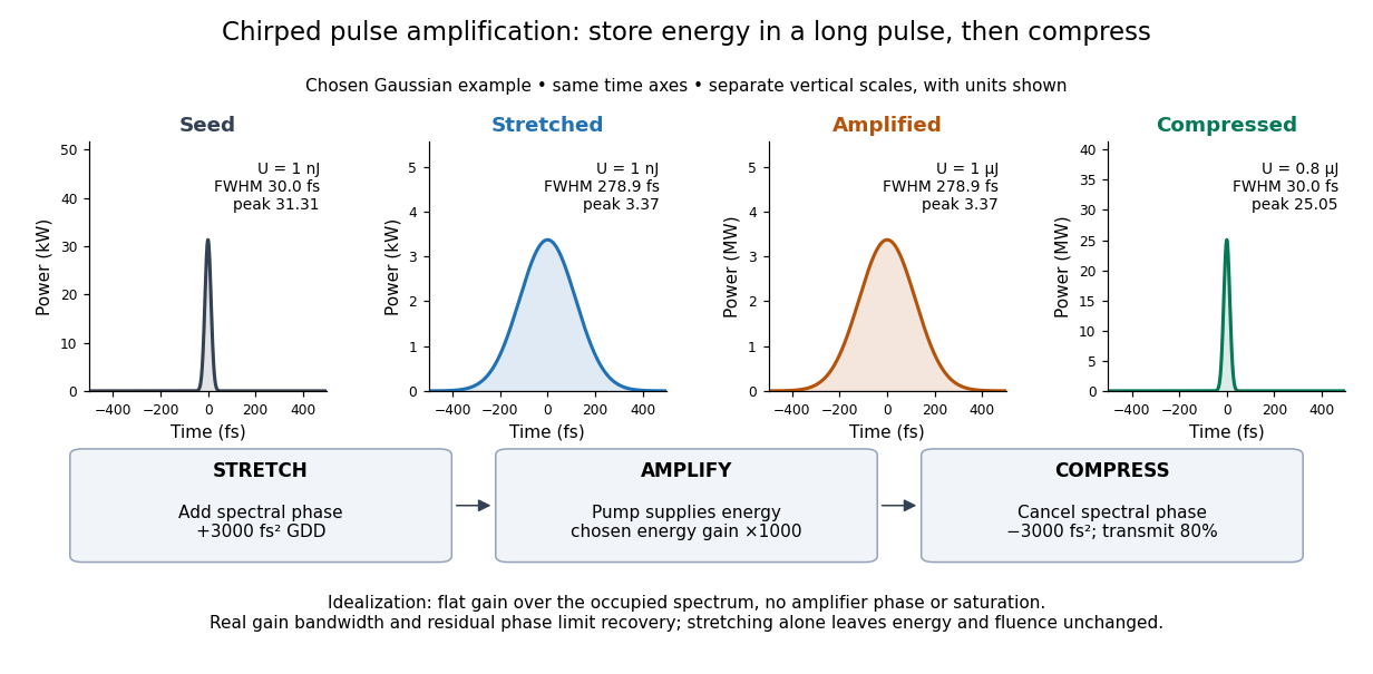
The useful idea is to arrange where the large peak power occurs. Lower light intensity in the amplifier reduces unwanted self-focusing and self-phase modulation; the compressed output can still drive strong nonlinear optics. Stretching does not remove every damage mechanism, and compression does not manufacture energy.
Let be the pulse's power integrated over its transverse section, and its energy. Its peak power is . For a chosen Gaussian power envelope with full width at half maximum ,The numerical shape factor is approximately . It matters when comparing quoted peak powers; the estimate assumes a shape and a width convention.
If an otherwise unchanged pulse is stretched by a factor without loss, its energy stays fixed and its peak power falls by . For energy gain and compressor energy transmission , ideal restoration of the original shape givesThese relations require a specified shape and preserved spectrum; they do not model amplifier saturation. For the diagram's chosen , seed, , and , the successive peak powers are , , and . The last pulse contains : the compressor increases peak power while losing some energy.
Fluence is time-integrated light intensity, , measured in . For a uniform beam of area , and . At fixed transverse profile, lossless temporal stretching lowers peak light intensity but leaves fluence unchanged. Absorbed energy, heat removal, beam size, coatings and pulse duration still constrain optical components. For nonoverlapping identical pulses at repetition frequency , the average power is ; it is a different quantity from peak power.
Use a complex envelope normalized so that ; its units are . The optical carrier convention is : the physical electric field is proportional to the real part of for a fixed transverse mode. With angular frequency offset , fix the Fourier transform conventionWrite with real . A dispersive element adds spectral phaseConstant phase rotates the envelope; the linear term delays it by . The group delay is . The quadratic coefficient is group delay dispersion, abbreviated GDD, with units of time squared. Positive GDD makes higher frequencies arrive later with this convention. It is accumulated dispersion of a component; material group velocity dispersion is its corresponding coefficient per unit length.
To undo a quadratic stretcher spectral phase, the compressor must supply opposite GDD. Include the amplifier and all intervening optics in the sum:Setting this sum to zero does not cancel third-order dispersion, , or still higher orders. Residual spectral phase can produce asymmetry and satellite pulses even when the quadratic term vanishes. A diffraction grating system can make path length depend on frequency; matching the complete spectral phase over the occupied spectrum is more demanding than merely choosing opposite quadratic coefficients.
There is a useful proof of what phase correction can accomplish. By Parseval's identity,For a smooth decaying spectrum, the Fourier transform of is . Consequently the power-weighted mean arrival time and variance obeyAt fixed spectral amplitude, constant group delay minimizes this root mean square duration. Such a pulse is a transform-limited pulse, up to a time shift and constant phase. The nonnegative second term measures temporal broadening from unequal arrival times; the first term remains even after perfect phase correction.
Choose an initially transform-limited pulse with Gaussian power and complex envelopeHere is the standard deviation of the power-weighted time distribution; is its full width at half maximum. Neither is a field-amplitude width. The spectral amplitude is proportional to , so the spectral power has standard deviation . The Gaussian time-bandwidth product in ordinary frequency is , where both widths are power FWHMs.
Multiplication by preserves spectral power and energy. Substituting into the moment identity givesThis is an exact result for a Gaussian spectrum with quadratic spectral phase. It also follows by completing the square in its inverse Fourier transform.
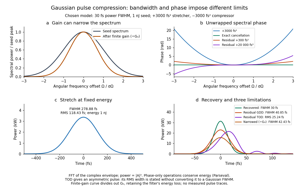
For these chosen inputs, . The stretched pulse has and root mean square width . Adding recovers ; leaving gives . All phase-only cases retain .
If GDD is cancelled but remains, the pulse is asymmetric. Gaussian spectral moments giveThus the centroid is and the root mean square duration is . Converting this last value to a FWHM with the Gaussian factor would be wrong: the power envelope is no longer Gaussian. The calculation's integrated energy agrees in time and frequency through Parseval's identity, while its centroid and variance agree with these independent moment formulas.
A real amplifier also changes spectral amplitude. For a simple small-signal example, stipulate an intensity gain profileThis specifies finite gain bandwidth, with no saturation or extra amplifier phase. Multiplying two Gaussian spectra givesFor chosen , the amplified spectrum is narrower by , the shortest Gaussian power FWHM becomes , and the total energy is . Perfect spectral phase correction cannot recreate the suppressed spectral amplitude. Real gain narrowing and saturation require a material-dependent amplifier model; a constant multiplier is only a limited idealization. Gérard Mourou's 2018 lecture discusses gain narrowing as a limit on the shortest amplified pulses.[ref]
Extreme Light Physics and Application by Gérard Mourou. Extreme Light Physics and Application, p.105, §II.E: finite gain bandwidth and gain narrowing
The 1985 experiment launched pulses from a mode-locked laser into of optical fiber. Dispersion and self-phase modulation produced a broader spectrum and approximately pulses. A Pockels cell selected a pulse for repeated amplification in neodymium glass, giving approximately before the double-pass diffraction grating compressor. Its transmission was 50 percent. The amplified output was reported as with a width limited by the streak camera response. The compressor was adjusted on fiber-output pulses using intensity autocorrelation; that measurement gave . Steve Williamson was acknowledged for help developing the concept, and Philippe Bado and Marcel Bouvier for technical support.[ref]
Compression of amplified chirped optical pulses by Donna Strickland and Gérard Mourou. pp.219–221, Figs.1–4 and acknowledgments: preparation, compressor adjustment, amplified readout and response limit
The crucial comparison is compression before and after amplification. It asks whether enough usable spectral phase structure survives the amplifier, rather than merely whether its output is bright. A response-limited trace cannot establish the true width below the detector's resolution or prove that every higher-order phase coefficient vanished. An intensity autocorrelation is also not a direct unique measurement of the complex electric field. These are limits on the inference, not extra controls attributed to the experiment.
Donna Strickland's 2018 lecture describes setting the compressor with the high-repetition oscillator pulses and making the amplified-pulse measurement with Steve Williamson's streak camera. It explicitly notes imperfect chirp matching.[ref]
Generating High-Intensity Ultrashort Optical Pulses by Donna Strickland. Generating High-Intensity Ultrashort Optical Pulses, p.168: separate autocorrelation and streak-camera measurements
The first apparatus therefore illustrates the strategy without establishing a universal lossless or exactly phase-matched amplifier.Donna Strickland leads an ultrafast laser group at Waterloo investigating intense laser interactions and nonlinear optics.[ref]
Donna Strickland by University of Waterloo. Biography and research interests: professional appointment and experimental research
Gérard Mourou's later work includes coherent combination of laser beams in the XCAN project at École polytechnique.[ref]The first laser pixels by École polytechnique. Professor emeritus and XCAN prototype: coherent combination of 61 beams
Their complementary research settings connect the original short-pulse experiment with the continuing problems of producing useful energy, peak power and average power together.Attosecond physics resolves changes on the scale of seconds, especially electron dynamics. Its central trick is to convert a short optical event into an experimentally accessible energy or phase change. A broad optical spectrum provides the ingredients for a short optical pulse; their spectral phases determine when those ingredients add constructively. High harmonic generation supplies the optical spectrum, while RABBITT and attosecond streaking supply complementary timing measurements. XUV denotes extreme ultraviolet radiation.
There are two separate timing problems: characterize the incident optical pulse, then infer the response of the target. A photoelectron measurement mixes the incident spectral phase, the target's transition response and the probing electric field. Recovering one requires constraints on the others. These methods measure distributions of photoelectron energies over repeated shots, rather than photographing a moving atomic orbital.
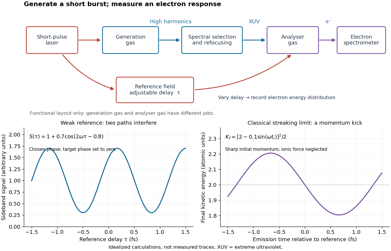
High harmonic generation converts an intense driving electric field into radiation at high integer multiples of its frequency. High harmonic generation in a gas is a process in nonlinear optics: an electron can leave a neutral target by tunnel ionization, gain kinetic energy in the driving electric field, and return to radiate upon recombination. This three-step picture is an approximate account of a probability amplitude for emission in quantum mechanics, not a measured path of one electron.[ref]
Generation and Measurement of Isolated Attosecond Light Pulses by Michael Hentschel. Generation and Measurement of Isolated Attosecond Light Pulses, slide 5: tunnelling, acceleration and return
Why odd multiples? In an ideal centrosymmetric gas driven by a single frequency, assume the radiating electric dipole moment satisfies , where is the driving period. Its Fourier series coefficient obeys , so every even coefficient vanishes. A finite envelope, an oriented target or an additional driving frequency can invalidate that symmetry argument. Producing many odd components also does not prove that their spectral phases form a short optical pulse.
The 1988 report involving Anne L'Huillier observed odd multiples of a driving wavelength in rare gases, reaching order 33 in argon. The unexpectedly slow fall of yield beyond the fifth order supplied a broad spectral plateau. A spectral observation alone did not establish the relative spectral phases needed for an attosecond pulse train.[ref]
Multiple-harmonic conversion of 1064 nm radiation in rare gases by M. Ferray and others. Multiple-harmonic conversion of 1064 nm radiation in rare gases, abstract
For an original classical calculation of the return step, neglect the residual ion's Coulomb force after release. Take a spatially uniform driving electric field , an electron of electric charge and mass , and zero initial position and velocity at . With and , integrating Newton's second law givesA return requires and . Define the cycle-averaged free-electron quiver kinetic energySearching the first-return solutions for release phases gives a maximum near and , with . For a chosen ionization energy , recombination into the initial state can therefore emit a photon with energy up to approximately in this model. This is an upper return-energy scale, not a prediction of the emitted yield. It omits release probabilities, quantum interference, propagation, phase matching and depletion of the neutral gas.
The calculation explains why a long driving wavelength can increase the available return energy: at fixed , grows as . It does not say that conversion efficiency improves. The electron must return with a probability amplitude for emission that survives the microscopic dynamics and adds coherently across the gas.
An attosecond pulse train contains repeated short optical pulses. For a group of odd multiples of a common driving frequency, the separation is half the driving period when the relative spectral phases recur. The construction resembles mode locking, but the participating components come from high harmonic generation, rather than separate resonant modes of a laser oscillator.
Choose equal-amplitude, monochromatic odd components with orders , , and odd . Fix the complex-field conventionHere is a normalized light intensity after averaging the fast carrier oscillations. Setting every and summing a geometric series givesAt the removable singularities take the continuous limit. Maxima repeat every ; the first zeros on either side of a maximum lie at . The zero-to-zero width is , which is not the full width at half maximum.
Choose orders and driving wavelength . Using with the speed of light gives and burst spacing . Solving the exact half-maximum equation gives a full width at half maximum of approximately attoseconds. These are values of the specified five-component model, not measurements from the 2001 experiment.
A deliberately chosen spectral phase translates the whole attosecond pulse train by without changing its shape. Adding makes neighboring phase increments unequal: the same component intensities then produce a different temporal profile. For the choice and radians per squared harmonic order, the adjacent-component delay estimates arenamely , , and for . This finite difference estimates the group delay at the pair's midpoint. It is not a single common arrival time.
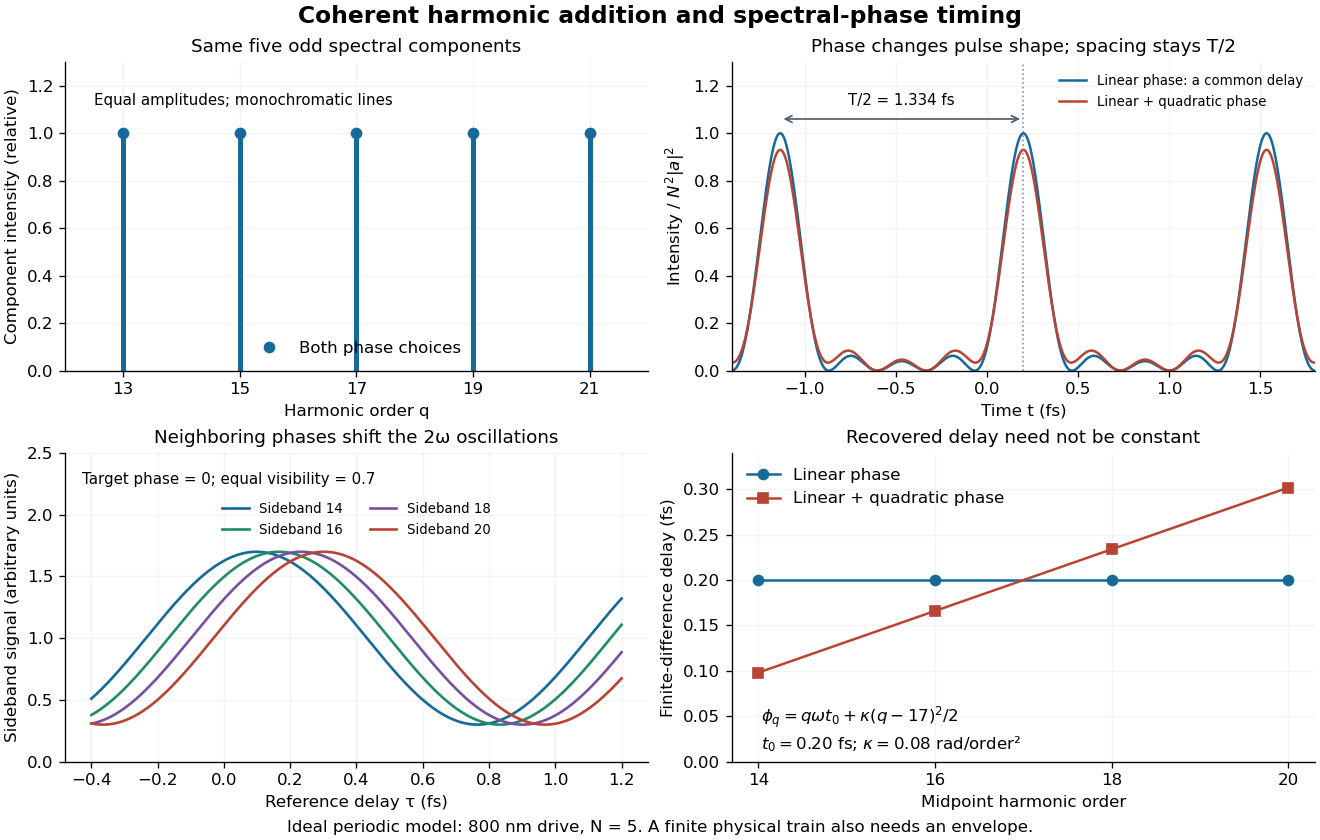
The infinite monochromatic sum is periodic forever and has infinite total energy. A real attosecond pulse train has a finite envelope and finite component linewidths. This calculation isolates coherent addition; it cannot describe an isolated burst or establish its contrast against satellites. As a further check, averaging over one half-period gives for any constant component spectral phases, because the cross terms integrate to zero by Fourier orthogonality. Spectral phase redistributes the light intensity in time while leaving that average fixed.
An isolated attosecond pulse has one dominant short burst within the observation window, with any satellite emission quantified. A broad optical spectrum alone cannot distinguish one burst from several. Selecting a generation interval and an appropriate spectral band can suppress neighboring bursts, but the resulting temporal contrast must still be tested.
For a simple calculation independent of any apparatus, let , with two nonoverlapping copies of a short optical pulse. Its optical spectrum has intensityA satellite produces spectral fringes of angular spacing when the two bursts are coherent and resolved. For chosen field-amplitude ratio , the satellite/main energy ratio is , while fringe visibility is . Weak satellite energy can thus leave substantial fringes. Averaging an uncontrolled removes the interference term without removing the satellite: absence of fringes alone does not prove isolation.
RABBITT measures adjacent harmonic spectral phases through two-photon photoionization. A weak delayed infrared reference opens two interfering paths to a shared photoelectron energy; the two-path attosecond phase reconstruction spells out the inference.
An original two-amplitude model makes the timing inference explicit. Use the spectral phase convention of the coherent harmonic pulse-train model, and define positive delay to retard the reference electric field. Let the amplitudes leading to the same final photoelectron state bewith real . Squaring their sum givesThe oscillation comes from opposite signs of the reference photon's phase. For and , the signal peaks at modulo . A fitted phase contains the target contribution ; setting it to zero is an assumption, not an observation. In an experiment, unobserved final channels can add as probabilities, so the displayed formula is one effective-channel idealization.
For a chosen example, impose radians and radians at . The observed oscillation has argument . Its peak shift is , while the corrected finite-difference group delay is . Ignoring the target contribution would bias the inferred delay by attoseconds. These stipulated phases demonstrate a reconstruction error; they are not atomic calculations or measured delays.
Recovering all neighboring phase differences determines the component spectral phases up to an overall phase and the chosen timing origin, provided the oscillation phases are consistently unwrapped. Known component amplitudes then give a temporal field by a finite inverse Fourier transform. This is why measuring the optical spectrum alone is insufficient: it omits the very information that decides when constructive wave interference occurs.
Pierre Agostini's experiment illuminated an argon jet with an annular beam. A pinhole removed the annulus; a tungsten-coated mirror relayed harmonics and weak central reference into another argon jet. A magnetic-bottle electron spectrometer used time of flight and microchannel plate detectors. Glass plates varied delay. Reference-on sidebands contrasted with reference-off peaks. Atomic-phase-corrected reconstruction yielded -attosecond bursts.[ref]
Observation of a Train of Attosecond Pulses from High Harmonic Generation by P. M. Paul and others. pp.1690–1691, Figs.1–4 and Table 1
The two-path attosecond phase reconstruction explains the control's purpose: adding the reference opens an interference channel. Its fitted oscillation tests phase relationships under the weak-field and atomic-response model. It does not independently reveal every target phase or an arbitrary nonperiodic optical pulse.
Attosecond streaking uses a synchronized reference electric field to change a photoelectron's outgoing momentum. Scanning relative delay produces an energy-versus-delay distribution. A short emission interval samples only a small part of the reference cycle; a longer interval samples a range of kicks and can broaden or reshape the distribution.
For an explicit classical limit, use the electric dipole approximation and choose the magnetic vector potential along the detection axis with and . Neglect the residual ion's Coulomb force. An electron released at with mechanical momentum obeysIndeed, integrating from release to the end of the field gives the stated minus sign. The useful clock variable here is , rather than the instantaneous itself. If is nearly linear across a narrow emission window with temporal standard deviation , and initial momentum is sharp, thenThis local mapping fails near a zero of , where first-order timing sensitivity vanishes. A real inversion must include the incident bandwidth, initial photoelectron distribution, collection angles and target–field response.
For an original dimensionless example in atomic units, choose , and . Then and , compared with initial kinetic energy . Reversing gives : the shifts are asymmetric because of the term. A measurement that keeps only the term linear in would miss in both cases.
The experiment involving Ferenc Krausz combined a subfemtosecond soft-X-ray pulse with a few-cycle visible electric field. Its delay-dependent krypton photoelectron spectra tested the field-controlled response. The reported pulse duration was attoseconds. Changing delay compared the emitted electron distributions at different reference phases; the spectral-width trace supplied a further duration-sensitive observable.[ref]
Attosecond metrology by Michael Hentschel and others. Attosecond metrology, abstract and Figs.3–5: krypton spectra, delay scan and width
The distinction from RABBITT is the measurement regime and reconstruction, rather than merely calling one trace a clock. The attosecond streaking momentum map is a limiting model; a finite-duration wave packet requires a quantum transition calculation. Inferring an emission delay also requires separating the illuminating pulse's spectral phase from the target response. The measurement supports time-dependent photoionization in a specified model, with no unique classical electron trajectory inside an atomic orbital implied.
Articles by others on the same topic

A laser is a device that emits light through a process of optical amplification based on the stimulated emission of radiation. The term "laser" is an acronym for "Light Amplification by Stimulated Emission of Radiation." Lasers produce coherent light, which means that the light waves are organized in a consistent phase relationship, resulting in a narrow, focused beam that can be very intense.



What makes lasers so special: Lasers vs other light sources.
How Lasers Work by Scientized (2017)
Source. An extremely good overview of how lasers work. Clearly explains the electron/photon exchange processes involved, notably spontaneous emission.
Talks about the importance of the metastable state to achieve population inversion.
Also briefly explains the imperfections that lead to the slightly imperfect non punctual spectrum seen in a real laser.
- youtu.be/_JOchLyNO_w?t=188 says LED is "also monochromatic", but that is not strictly true, it has way way larger frequency band than a laser. Only narrower compared to other sources such as incandescent light bulbs.
- youtu.be/_JOchLyNO_w?t=517 stimulated emission. This is the key to laser formation as it produces coherent photons.
- youtu.be/_JOchLyNO_w?t=581 spontaneous emission happens too fast (100 ns), which is not enough time for stimulated emission to happen. Metastable electrons to the rescue.
- youtu.be/_JOchLyNO_w?t=832 the parallel mirrors select perpendicular photons preferentially