Fluorescence is photon emission following photon absorption by matter: an excited state releases some of its energy as light. A fluorophore can therefore mark where something is, while its fluorescence emission spectrum and fluorescence lifetime report different aspects of its environment. Fluorescein is one example; FRET exploits a competing route for excitation energy rather than requiring a second emitted photon.
The usual molecular sequence is excitation, relaxation, then emission, as in the Jablonski diagram. The emitted photon commonly has lower energy and longer wavelength, giving a Stokes shift; the exceptions are discussed below.[ref]
What is the Stokes Shift? by Edinburgh Instruments. Stokes Shift in Fluorescence Spectroscopy, Figure 4 and relaxation discussion
Blue fluorescence of suitably acidified quinine solutions, used in identifying quinine and illustrating fluorescence.
The precision of a fitted single-emitter position is distinct from its diffraction-broadened point spread function width. An ideal Gaussian function image of width with independent detected photons gives . Pixel size, background, model error, sample motion and drift limit practical performance; precision alone does not guarantee accuracy.[ref]
Precise nanometer localization analysis for individual fluorescent probes by Russell E. Thompson and others. Localization uncertainty with finite photon number, pixelation and background
For a compact cloud passing a stationary source at distance , put and . Incoming and returning rays have opposite Doppler factors. Source return time is . If , line-centre excitation is possible above and occurs at closest approach when . In a weak, optically thin, isotropic spontaneous emission model, the excited population obeys and the received bolometric intensity scales as . Finite lifetime and line width smear the pulse and its frequency chirp; geometry and source strength are needed for an absolute prediction.
Spectroscopy measuring emitted light following excitation. Emission peak position and intensity can report changes of speciation, but concentration, excitation absorption and photochemical loss also influence the signal.
Fluorescence emitted by intrinsic sample components, which can contribute background in a labeled assay.
fluorescence recovery after photobleaching follows fluorescence return to a bleached region as unbleached labeled molecules redistribute. Recovery depends on geometry, transport, binding and immobile fractions; it is not a direct measurement of every aspect of membrane fluidity.
fluorescence anisotropy measures the polarization dependence of emitted fluorescence after polarized excitation. It can constrain rotational freedom on the fluorescence-lifetime timescale, but probe orientation, lifetime and partitioning also affect the signal.
fluorescence correlation spectroscopy analyzes fluctuations of detected fluorescence to infer quantities such as molecular number and movement through an observation volume. Photophysical fluctuations and background must be distinguished from transport.
A reduction in fluorescence caused by a process competing with photon emission, for example a collision that removes excitation energy without emitting a photon. Measuring less light because fewer excitation photons reach the sample does not by itself establish fluorescence quenching.
Loss of fluorescent population through nonemitting ground-state association. In a simple static-only case the surviving unbound emitters keep their lifetime, distinguishing it from dynamic quenching; mixtures and association-dependent spectra complicate that test.
Quenching by an excited-state encounter that introduces an additional decay rate . It reduces both fluorescence quantum yield and lifetime in the simple single-population model.
For purely dynamic quenching of a single emitting population, . The slope measures , so determining a bimolecular quenching constant requires the unquenched lifetime or equivalent independent rate information.
An increase in fluorescence caused by reducing a quenching interaction. Dye dilution can reduce Förster resonance energy transfer; the signal alone need not identify the process that diluted the dyes.
A fluorophore is a fluorescent molecule or fluorescent part of a molecule. Its usefulness as a label depends on how efficiently it absorbs the chosen excitation light, its fluorescence quantum yield, and its resistance to photobleaching. A large fluorescence quantum yield alone does not guarantee a bright image if few excitation photons are absorbed or collected.
A Jablonski diagram arranges molecular energy eigenstates vertically and draws arrows for changes between them. In the usual closed-shell molecular example, is the electronic ground state, and are electronic excited states with singlet state spin, and has triplet state spin. Each electronic state also has levels of molecular vibration. The diagram records possible processes, not molecular paths in space.[ref]
Photon absorption can populate an upper level of molecular vibration in . Relaxation removes excess energy without photon emission; fluorescence commonly starts from relaxed .[ref]
What is the Stokes Shift? by Edinburgh Instruments. Stokes Shift in Fluorescence Spectroscopy, Figure 4 and its discussion
The drawing also includes relaxation from a higher electronic excited state and a competing spin-changing route to a triplet state.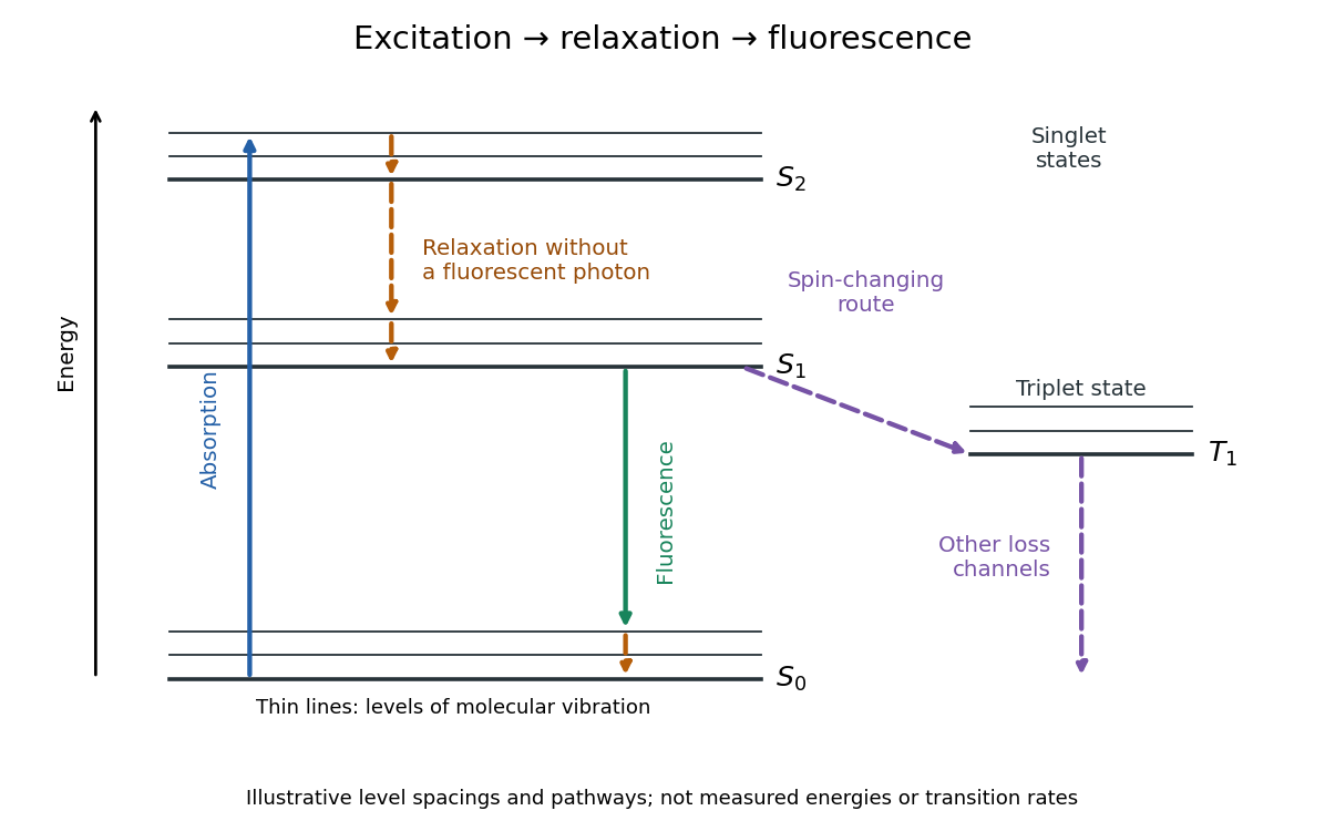
The Stokes shift compares the lowest absorption-band maximum with the fluorescence emission spectrum maximum. Relaxation often makes . This comparison differs from using an arbitrary excitation wavelength. A spectral-density maximum can move when changing from per unit wavelength to per unit spectroscopic wavenumber; specify the spectral convention.[ref]
What is the Stokes Shift? by Edinburgh Instruments. Stokes Shift in Fluorescence Spectroscopy, definition, spectral-coordinate caveat, Figures 2 and 4
An original illustrative energy budget makes the distinction concrete. Excitation at and emission at correspond to about and per photon, using with Planck constant and speed of light in vacuum. The difference, about , must go elsewhere in the complete energy balance. These chosen wavelengths are not measured band maxima for a particular fluorophore.
Anti-Stokes emission has shorter wavelength than excitation. Additional energy, for example from a thermally populated level of molecular vibration or multiple excitation photons, makes it possible. The one-photon, initially relaxed drawing does not cover these cases.[ref]
Advanced Fluorescence Microscopy Techniques—FRAP, FLIP, FLAP, FRET and FLIM by Hellen C. Ishikawa-Ankerhold and others. §1.1.1, final paragraphs: anti-Stokes emission and multiphoton excitation
A fluorescence excitation spectrum scans excitation wavelength while detecting fluorescence in a fixed emission band. A fluorescence emission spectrum does the converse. The inspected spectrofluorometer example uses an excitation monochromator scan with the emission monochromator fixed, and reverses their roles for emission.[ref]
An operational model explains why this need not reproduce absorption. For one dilute, unsaturated emitting species, write for absorbed fraction, for incident photon rate, for fluorescence quantum yield, and for the fraction of emitted photons counted in the selected band. The background-subtracted count rate isOnly after correcting incident photon rate, and with constant yield and emission-band collection, is this proportional to absorbed fraction. A nonfluorescent absorber contributes to absorption but not this readout. Thick samples, multiple emitting species, and reabsorption of fluorescence complicate the model.
A fluorescence emission spectrum resolves emitted photons by wavelength at fixed excitation settings. Subtract a matched sample-container and solvent background, and correct the wavelength-dependent throughput and photodetector sensitivity when estimating the emitted distribution. A camera image through one fluorescence emission filter instead measures a weighted band integral, not a whole fluorescence emission spectrum. A fluorescence lifetime resolves delay after excitation; its horizontal axis is time, not wavelength.
Fluorescence quantum yield counts emitted fluorescent photons per absorbed excitation photon. It differs from quantum efficiency, which describes the photodetector.[ref]
For an original constant-rate model, let be the radiative decay rate and the sum of competing rates without fluorescent photon emission. An initial population in the emitting excited state obeys the rate equationIntegrating over all time givesHere every absorbed excitation is assumed to reach this emitting population; additional losses before that stage require another factor. Under steady weak excitation, absorbed photon rate and total detection fraction give . The count rate therefore mixes excitation, yield, and detection, whereas specifies a decay timescale.
Photobleaching is an irreversible loss of fluorescent capacity caused by illumination. It changes the number of active fluorophores over experimental time; fluorescence lifetime concerns the delay after an individual excitation. Reversible dark states and ordinary return to the ground state are different processes.
In a stipulated population-loss model, let denote elapsed illumination time and denote delay after a pulse. If active population declines as while surviving fluorophores retain the same decay rates, then . Brightness falls while stays fixed. This example does not assert that all bleaching follows exponential decay: chemical changes and selective loss from a mixture can also change the observed decay shape. The existing FRET photobleaching controls illustrate why deliberate bleaching requires careful interpretation.
Two initially active independent emitters with exponential lifetimes of rate have last-bleaching time . Independence gives for . Differentiating proves the density in the title, and integrating its survival function gives . The first event has rate , while the waiting time from first to second has rate .
For the constant-rate model in fluorescence quantum yield, fluorescence lifetime is the mean residence time in the emitting excited state and the timescale of its exponential decay. The detected fluorescent photon rate after an ideal instantaneous pulse is for . Its amplitude and its decay timescale are separate quantities.
For a stipulated example, rates give and . Rates give the same but . Conversely, doubling doubles the ideal amplitude without changing . Equal fluorescence lifetimes need not imply equal brightness or equal fluorescence quantum yields.
Different environments can supply several populations, giving rather than one exponential decay. A fitted single timescale then depends on the selected model and detection band. FRET donor lifetime uses the change in a donor's decay when transfer introduces an additional loss route; the FRET branch develops that interpretation.
A fluorescence instrument response is the distribution of recorded delays for an effectively prompt optical signal. Finite excitation-pulse width and timing variation in the photodetector and electronics contribute. With a normalized response , intrinsic fluorescent photon rate , and background rate , the expected trace isFit a candidate decay after this convolution with the measured response; treating the broadened leading edge as the intrinsic decay can bias fluorescence lifetime. The accessible technical note describes measuring prompt scattered excitation with a nonfluorescent scattering sample.[ref]
Time-Correlated Single Photon Counting (technical note v. 2.1) by Michael Wahl. Michael Wahl, Time-Correlated Single Photon Counting, v. 2.1, p. 3: scattering-medium response measurement and iterative reconvolution
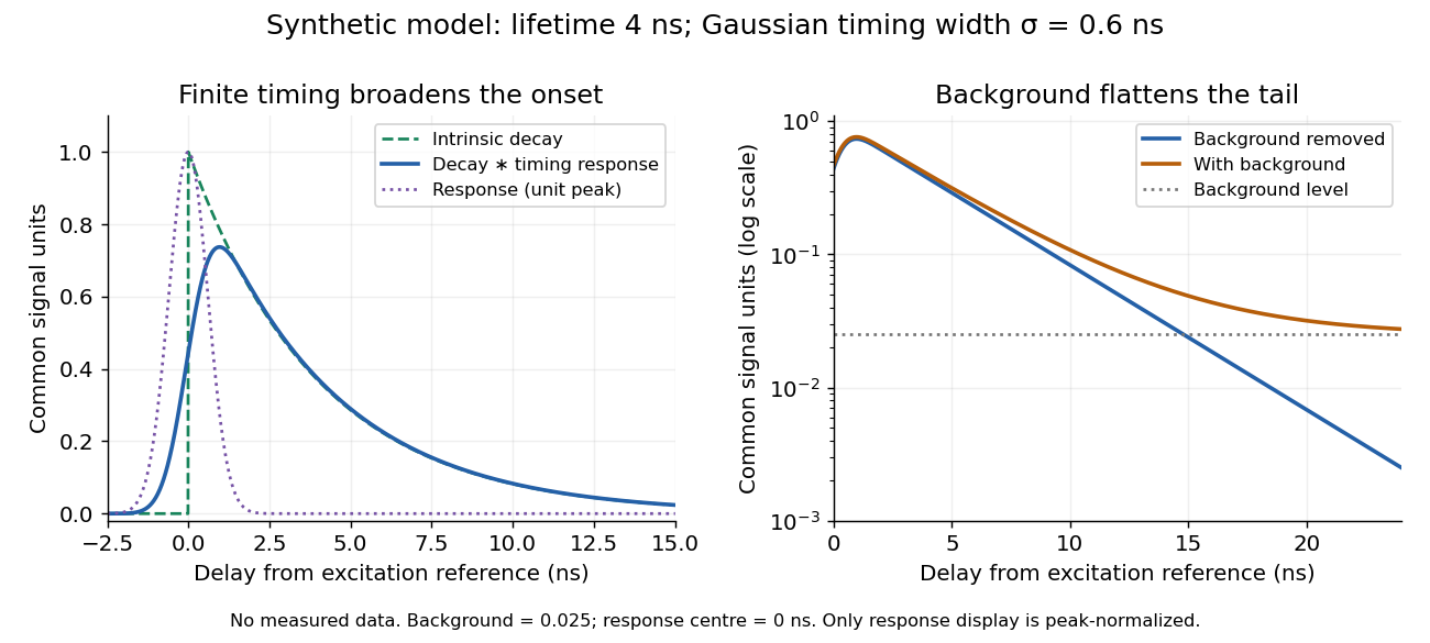
Synthetic fluorescence lifetime decay broadened by an instrument response
. Original stipulated model, not measurements: for and zero otherwise; is a normalized Gaussian function of standard deviation centred at zero; the background is in the common signal units. The left panel compares intrinsic and convolved traces; the right shows how an unremoved background flattens the tail on a logarithmic scale. Negative delays come from the stipulated timing response about the pulse reference, not emission before excitation. Only the instrument-response curve is rescaled to unit peak for display. Details.The inspected apparatus sends picosecond diode-laser pulses into a sample cuvette. A neutral attenuation filter keeps detected events rare; an emission cut-off filter rejects scattered excitation. Collection optics deliver fluorescence to a photodetector; detector pulses and the laser-driver synchronization signal feed the timing electronics. The illustrated arrangement uses a PDL 800-B driver and TimeHarp 200 electronics. The note's recorded comparison uses two dye solutions and a prompt instrument-response trace; the dye tails have distinct slopes on a logarithmic display. Its Figure 9 measurement specifies an 80 MHz source, separately from the Figure 8 driver-setting example.[ref]
For a defensible new measurement, separately acquire detector background with excitation blocked, a solvent/container blank under excitation, and a prompt response appropriate to the timing channel. Compare successively attenuated acquisitions to expose pile-up; compare early and late acquisition intervals to expose photobleaching. Choose a repetition period long enough for the relevant decay or include residual population from earlier pulses in the model. These are proposed checks, not additional controls claimed for the published curves. Photon shot noise, background mismatch, and uncertainty in the fluorescence instrument response limit how uniquely multiple decay components can be inferred.
A fluorescence microscope maps photon emission to an image. Excitation light passes through a fluorescence excitation filter and reflects from a wavelength-selective beam splitter into the objective optical lens. Returning fluorescence passes through that beam splitter and a fluorescence emission filter to the photodetector. Rejecting excitation makes faint emission visible.[ref]
Advanced Fluorescence Microscopy Techniques—FRAP, FLIP, FLAP, FRET and FLIM by Hellen C. Ishikawa-Ankerhold and others. §1.2.1, Figure 5 and excitation/emission-filter paragraphs
An ordinary image records emission-band counts at each pixel. Adding pulse-delay measurements gives a fluorescence lifetime map; scanning emission wavelength gives spectral information instead. Confocal microscopy adds spatial rejection and confocal optical sectioning, as developed in its own branch. An unlabeled specimen under the same illumination reveals intrinsic fluorescence and excitation leakage; excitation-blocked frames reveal detector background. A blank cannot perfectly predict background in a differently prepared specimen.
Fluorescence measurements resolving individual labelled molecules or molecular events, allowing heterogeneous dynamics to be distinguished from population averages.
Uncertainty in an estimated emitter position. It can be much smaller than the width of its point spread function, but it does not by itself guarantee that densely packed emitters or an entire labelled structure are resolved.
fluorescence microscopy forms images from spatially resolved fluorescence. Probe partitioning, optical resolution and photophysics constrain what a fluorescent pattern establishes about molecular composition or contact.
Live-cell imaging follows living biological cells over time. Labels, illumination and immobilization must be checked for effects on the process being measured; an apparently sharp image is not sufficient evidence that the cell remains physiologically unperturbed.
Imaging of biological events in a living organism. Repeated cell tracking can establish event ordering but requires controls for phototoxicity, imaging access and sampling.
An illumination-induced change in a fluorescent label that allows a selected cell or region to be distinguished and followed over time.
Biological damage caused by illumination, which can alter development even when an image remains visually clear. Non-imaged and dose-matched controls help identify it.
A fluorescence microscope technique that illuminates a thin plane and detects emitted light from another direction, enabling repeated optical sectioning of living specimens.
A fluorescence excitation filter selects the illumination wavelength band reaching the specimen. Its finite transmission changes the absorbed photon rate and thus image brightness. Specify that band when interpreting a fluorescence excitation spectrum or comparing images.
A fluorescence emission filter transmits the chosen emitted wavelength band while rejecting excitation leakage. Finite rejection, overlap of the fluorescence emission spectrum with excitation, and the photodetector's wavelength-dependent response can all affect the count. A darker filtered image alone does not establish a changed fluorescence lifetime or increased photobleaching.
Confocal microscopy forms an image by scanning a localized illumination spot and preferentially detecting light from the same small region. In a thick specimen emitting fluorescence, a conventional fluorescence microscope also collects a haze from material away from the selected optical focus. Confocal optical sectioning suppresses that haze, revealing structure at a chosen depth without cutting the specimen. The useful idea is a paired selection: where excitation occurs, and which emitted photons reach the photodetector. [ref]
Introductory Confocal Concepts by Nikon Instruments Inc.. Introductory Confocal Concepts, opening paragraphs and Fig. 2: out-of-focus fluorescence and optical sections
The scope here is single-point, linear fluorescence imaging. Confocal microscopy can also use reflected light; its broader implementations need not all have the same scanning mechanism. The patent Microscopy apparatus, US3013467A, by Marvin Minsky describes a point source imaged onto a specimen, a second pinhole receiving its image, specimen scanning, and a synchronized display. It was filed on 7 November 1957 and published on 19 December 1961; the filing date should not be described as the grant date. This is evidence for that apparatus and those dates, rather than a claim that all later fluorescence instruments were already present in it. [ref]
Microscopy apparatus by Marvin Minsky. Front-page filing/publication metadata; description, Optical System, Fig. 1; Stage Scanning System
Two planes are optically conjugate when an optical lens system images one onto the other. In confocal microscopy, an illumination pinhole is imaged onto the selected specimen point, and that specimen point is imaged onto the detection pinhole. Thus the two apertures select corresponding positions in different planes; they need not occupy the same physical plane. Modern laser instruments can supply the illumination point with an optical fiber or a suitable focused laser mode instead of a separate metal illumination pinhole. [ref]
Confocal microscopy (chapter manuscript) by Brad Amos and others. Amos, McConnell and Wilson, Confocal microscopy, manuscript pp. 5, 7–8: conjugate foci, Fig. 3, fiber-delivered illumination
A fluorescent emitter at the selected optical focus forms a compact point spread function at the detection aperture. An emitter displaced axially produces a broadened spot there through defocus; a smaller fraction of its collected light passes. The emitter still exists and still emits photons. Rejected photons strike the opaque mask or other parts of the instrument instead of contributing to the accepted detector channel. Neither a finite pinhole nor diffraction makes the accepted out-of-focus contribution exactly zero.
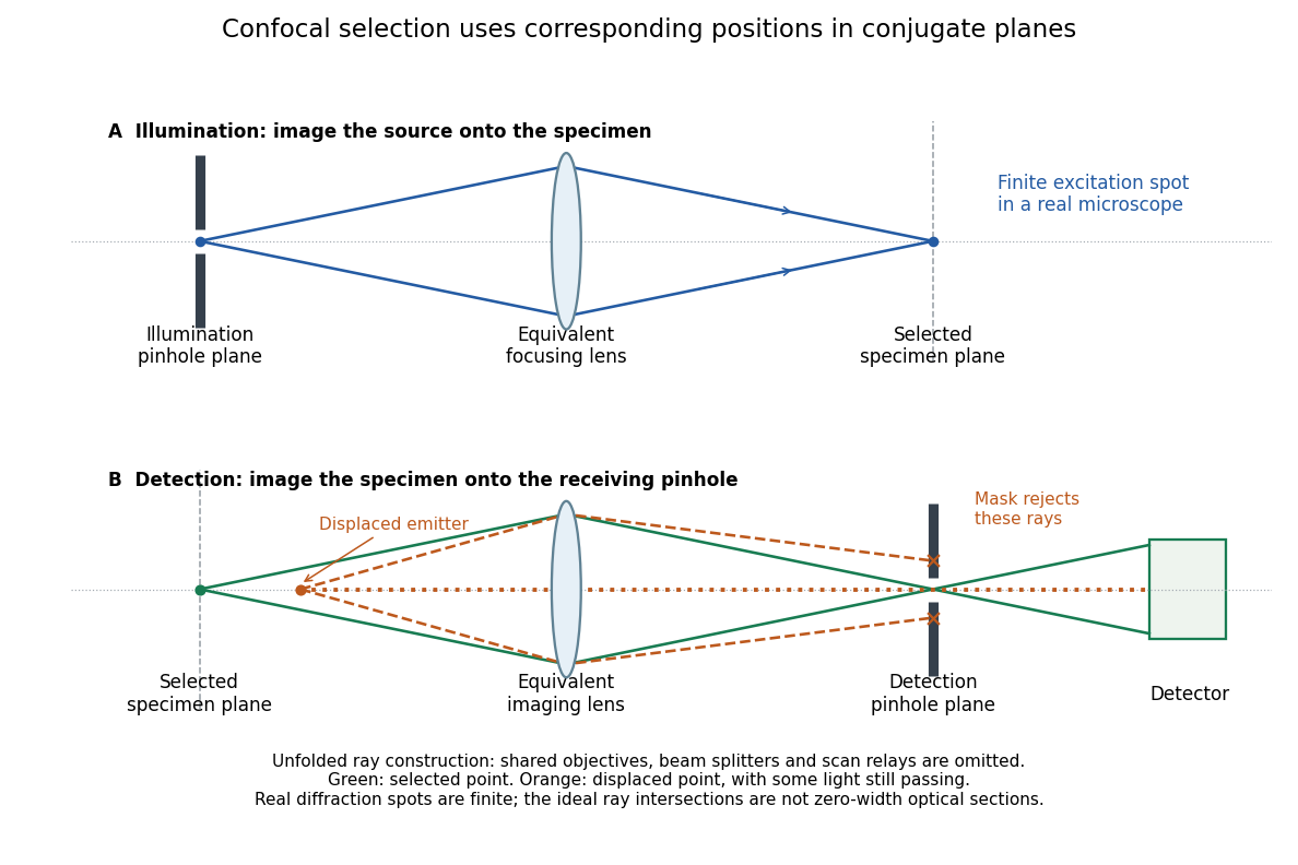
Conjugate illumination and detection pinholes in confocal microscopy
. Original unfolded geometrical optics schematic, not a scale drawing of an instrument. The top panel images an illumination pinhole onto the specimen; the lower panel images the selected specimen point onto the detection pinhole. Dashed orange light rays from an axially displaced point strike the mask, while an axial orange light ray passes. Real spots have finite point spread functions through diffraction; the drawing's perfect green intersection is only a ray construction. A fluorescence instrument may fold both paths through the same objective optical lens using a wavelength-selective beam splitter. Details.At one depth, scan the illumination spot across and and assign the detector reading during each dwell interval to a pixel. Move the specimen or objective optical lens axially to acquire the next depth. A stack of these optical sections samples three-dimensional structure. With beam scanning, the returning fluorescence commonly retraces the scanning optics: this descanning holds the image of the currently illuminated point at the detection pinhole. With stage scanning, the fixed spot and pinhole remain aligned while the specimen moves. [ref]
An optical section is a depth-weighted image of an intact specimen, with a finite axial response and tails. A physical cut actually separates a slice of material; its thickness and cutting damage are properties of the preparation. Changing optical focus selects another optical section without removing a slice, although illumination can still damage a specimen. Neither a thin physical slice nor a sharply displayed optical section makes the imaging point spread function infinitely narrow. [ref]
Introductory Confocal Concepts by Nikon Instruments Inc.. Fig. 2 discussion: focused-light sections rather than physical sectioning
Point response and section thickness answer different questions. For a spatially uniform, very thin fluorescent sheet, its response versus axial displacement is proportional to the lateral integral of the three-dimensional confocal response,Consequently a trace through a single bead, , does not by itself give the sheet's optical-section thickness. State which object and which full width at half maximum are being measured. A smaller axial sampling step gives more samples of the same response, rather than automatically improving diffraction-limited resolution. [ref]
Confocal microscopy (chapter manuscript) by Brad Amos and others. Appendix §6, manuscript pp. 42–43: thin fluorescent sheet translated through focus
For an isolated fluorescent molecule at displacement from the scanning optical focus, write for relative excitation light intensity and for the fraction of its collected emission passed by a centred detection pinhole of radius . The expected response, apart from a common brightness and collection factor, isHere is position in the detection-pinhole plane and is the emitted light intensity distribution there conditional on collection, with units of inverse area. This point spread function normalization retains throughput: is a fraction, not a curve rescaled to have peak one. The product expresses excitation followed by detection; it is an intensity/probability product, not multiplication of coherent wave amplitudes from different molecules. [ref]
Confocal microscopy (chapter manuscript) by Brad Amos and others. Manuscript p. 16, Fig. 4 discussion; Appendix §5, p. 37, Eq. A17: illumination-times-detection response
Assume linear, unsaturated fluorescence, independent emitters whose light intensities add, a stationary specimen, fixed collection efficiency and quantum efficiency, and negligible changes from scattering, absorption or bleaching during a scan. Different excitation and emission wavelengths generally give different excitation and detection responses. For a sufficiently small pinhole, is approximately its area times at the centre; this is the familiar excitation-times-detection point spread function. It is not universally the square of one point spread function. A spatially invariant response further allows the image to be expressed as a convolution with the emitter distribution; depth-dependent optical aberrations can invalidate that approximation.
For an explicitly synthetic axial example, put and choose an on-axis excitation , inspired by a Gaussian beam. Stipulate a circular Gaussian function for the detection-plane light intensity, with standard deviation . In dimensionless coordinates , put . ThenThe expression for follows by integrating over a disk using polar coordinates. The assumptions specify a toy model with matched axial scales; its parameters are not a calibration for a real objective optical lens. It omits Airy disk rings, vector diffraction, and unequal excitation and emission wavelengths.
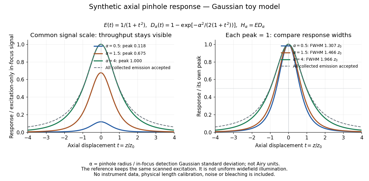
Synthetic axial response: narrower pinholes reduce throughput and suppress defocus
. Original Gaussian toy model, not measurements. The left panel keeps a common signal scale; the right divides each response by its own peak to compare widths. Here is a radius in units of detection-plane Gaussian standard deviation, not an Airy-unit diameter. The dashed reference is the same scanned excitation with all collected emission accepted, not conventional uniform widefield illumination. Both panels retain nonzero out-of-focus tails. Details.For a vanishingly small pinhole, the peak-normalized synthetic response tends to , whose full width at half maximum is . With all collected emission accepted it tends to , of width . Meanwhile as the pinhole closes. The narrower normalized curve therefore accompanies a vanishing detected signal; peak normalization must not conceal that loss.
Opening the pinhole increases accepted in-focus and out-of-focus photons; closing it strengthens confocal optical sectioning while discarding some useful in-focus photons too. In the synthetic model, transmits approximately of the collected in-focus emission. At the corresponding peak-normalized signals are about . These are calculated fractions under stated assumptions, not instrument measurements.
An Airy unit conventionally specifies a pinhole diameter equal to the first-zero diameter of the emission Airy disk in that plane. For an ideal circular pupil,where is the total specimen-to-pinhole magnification, the emission wavelength in vacuum, and the objective numerical aperture. A software setting needs its specified wavelength and relay magnification; it is not a universal micrometre diameter. [ref]
Confocal microscopy (chapter manuscript) by Brad Amos and others. Appendix §6, manuscript pp. 42–43: Airy unit defined between the focal spot's zeros and conversion to real units
For ideal independent counting, accepted source and background means and give photon shot noise with variance and signal-to-noise ratio in photon counting . Closing a pinhole need not improve that ratio: it depends on how both and change. Increasing exposure or excitation to replace discarded photons can cause bleaching, an irreversible loss of fluorescent emission capacity, or damage. Detection rejection occurs after excitation and therefore does not undo excitation outside the selected depth. Such material can absorb illumination and emit photons even when their emission is omitted from the recorded image.
A useful motivating experiment moves a bead emitting fluorescence through the selected optical focus and records the detector signal against position. Measurement of point-spread function (PSF) for confocal fluorescence microscopy by InCheon Song and others (2005, §2 and Fig. 1) describes a laser delivered through a single-mode optical fiber, collimation, beam-size adjustment and a dichroic beam splitter. A , numerical aperture oil-immersion objective optical lens excites slide-mounted fluorescent beads and collects their emission. Emission passes a filter and collecting optical lens, then a pinhole, before an avalanche photodiode. A three-dimensional positioning stage moves the specimen. The apparatus also contains a phase plate for deliberately modified responses.[ref]
Measurement of point-spread function (PSF) for confocal fluorescence microscopy by InCheon Song and others. §2 and Fig. 1, pp. 2–3: apparatus and readout
The published comparison uses nominal bead diameters : larger beads give broader measured spots. This is a control on the finite emitter, because the image is the convolution of bead emission with the confocal point spread function. The smallest bead has weaker signal relative to noise; incorrect bead size, defocus, bleaching and optical aberrations limit inference from a restored response. The reported bead-size comparison concerns lateral responses; it is not a measured pinhole-size series or a measured sheet-sectioning curve.[ref]
To test axial pinhole selection with this kind of apparatus, the following is a proposed extension, not an additional result from that paper. Choose an isolated bead small relative to the response, centre it laterally, then step through optical focus while recording background-subtracted signal at several pinhole settings. Hold excitation power, dwell interval, detector gain, emission band and sampling fixed. Preserve raw peaks before also plotting peak-normalized traces. A lower peak and faster relative decay with axial displacement would support the paired-selection mechanism; fitting only normalized widths would miss the throughput cost.
Measure blocked-excitation background, include a bead-free region, avoid detector saturation, and repeat scans in reversed order to reveal drift or bleaching. Check pinhole centring separately, since misalignment can mimic signal loss. Record bead diameter, immersion medium, refractive index, numerical aperture, wavelengths and axial step. A finite bead is an approximation to an optical point source; a point trace does not certify confocal optical sectioning of a whole fluorescent sheet. Depth-dependent spherical aberration, scattering and sample motion can broaden or distort the response. Increasing magnification or making a display brighter does not correct those effects.
Immunofluorescence localizes antigens using antibodies and a fluorescence readout. Indirect labeling uses a secondary antibody to detect the bound primary antibody.
A screen whose fluorescence makes the spatial distribution of incident electrons or other radiation visible.
Articles by others on the same topic

Fluorescence is a process in which a substance absorbs light or other electromagnetic radiation and then re-emits light. Specifically, it refers to the emission of visible light by a substance that has absorbed ultraviolet or other high-energy radiation. The process usually occurs very quickly, typically within nanoseconds.