 Q-Q plot

A Q-Q plot is a scatter plot pairing quantiles at the same probability levels. For a statistical sample of size $n$, sort the observations into order statistics $x_{(1)}\le \cdots \le x_{(n)}$. Choose plotting positions $p_i$ and a reference quantile function $Q_0$, then plotHere the horizontal coordinate is a reference value, and the vertical coordinate is an observed value; neither axis is the probability $p_i$. The displayed plotting positions are our chosen convention, placing every level strictly between zero and one. They are not a claim that the $i$th order statistic equals that population quantile. For two statistical samples, use sample quantiles at matching levels, with a stated interpolation convention when their sizes differ. ^[ref]

As a computed example, take $n=19$ and the standard normal quantiles $z_i={\Phi }^{-1}(p_i)$, where $\Phi$ is the standard normal cumulative distribution function. Construct the ordered values $a_i=10+2z_i$. At ranks $1,10,19$, the plotting positions are $1/38,1/2,37/38$, the reference quantiles are approximately $-1.937932,0,1.937932$, and the constructed values are approximately $6.124137,10,13.875863$. Every point lies on $a=10+2z$ by construction. These 19 values are deliberately chosen, not random draws or real measurements.

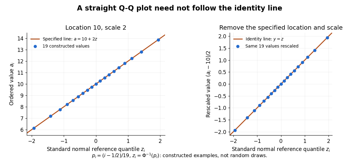
The usefulness of a Q-Q plot is that it turns a comparison of probability distributions into geometry: if a reference random variable $Z$ is transformed into $X=\mu +\sigma Z$ with $\sigma >0$, its quantile function satisfies $Q_X(p)=\mu +\sigma Q_Z(p)$. This follows because a positive scaling preserves ordering. Thus the location-scale family produces a straight population Q-Q plot, and an approximate sample line suggests a compatible shape over the observed range. Its intercept describes location and its slope describes scale. The identity line requires the same location, scale and units on both axes; even then its displayed angle is 45 degrees only with equal axis scales. Curvature is often more informative than a histogram because it shows which quantiles depart from the reference. ^[ref]