
Resting cells enter proliferation at rate . A proliferating cell takes a fixed cycle time to divide and survives that cycle with probability under a constant death hazard . Thus exit from the proliferating compartment at time is , and it returns twice as many daughter cells to the resting population. Resting-cell loss at rate is separate.
More explicitly, the number currently in the proliferating stage isfor a consistent initial history. Differentiation gives the stated equation. Counting resting-cell entry, loss and daughter-cell return gives its equation. Negative feedback in suppresses recruitment when the resting population is high; its Hill exponent gives a steep response around the concentration scale .
Set and defineThen , so the resting-cell equation becomes exactlyThe nonzero steady state solves , or for positive . The latter right side decreases strictly from to zero. Thus when there is exactly one positive equilibrium,Zero is also an equilibrium; negative populations are outside the biological domain. The same result is visible by intersecting the line with the hump-shaped .
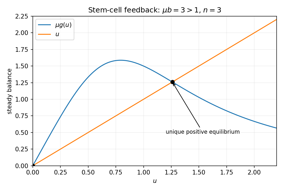
Resting-cell recruitment feedback has one positive equilibrium when the small-population reproduction factor exceeds one
. Details. 
Put . Linearization and a mode giveHere is the coefficient called in the source's characteristic equation; it is not the proliferating-cell death hazard. Any characteristic root with positive real part makes the equilibrium linearly unstable. A nonzero imaginary crossing satisfies and ; these are its Hopf conditions, subject to nondegeneracy.
On slow time , the unit delay becomes . Taylor expansion gives . Dividing the equation by therefore yieldsThis approximation requires slow smooth variation and a denominator bounded away from zero; a vanishing denominator marks failure of this slow reduction. On the fast time , omit only the explicit order- terms, retaining the finite delay:Replacing the delayed argument by the present value on that fast scale would incorrectly erase the dynamics. These are the slow and fast limits of a delayed stem-cell model.
The decreasing production term represents negative feedback: low red-cell abundance stimulates production, whereas high abundance suppresses it. The linear loss term models removal at constant per-cell rate. SetThen , with . On the physical half-line , decreases from one to zero while increases from zero to infinity. Their unique intersection is the steady state. Its linear derivative is , so it is asymptotically stable.
For small , the intersection lies at large , where ; for large it lies at small , where . HenceImplicit differentiation of gives . The plot joins these two decreasing asymptotic regimes.
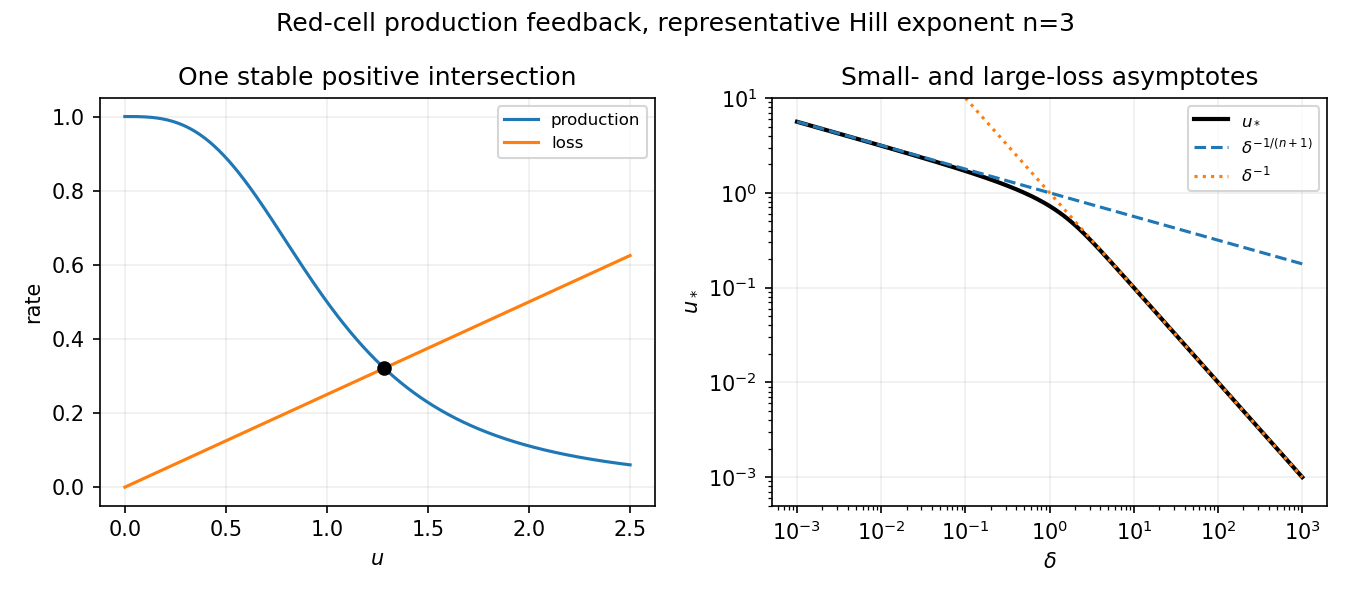
Negative production feedback gives one stable red-cell equilibrium and two limiting concentration scalings
. Details. 
The delay represents the time between feedback sensing and the appearance of newly produced mature cells. In dimensionless time it is , so the equation becomesIt requires a nonnegative initial history on , not just one initial value. Its constant equilibrium is unchanged. Put . A small perturbation obeys , whose characteristic equation isThere is no real root with , because all three terms would have positive sum; zero is never a root either. Starting from the stable zero-delay case, loss of linear stability can therefore occur only when a complex conjugate pair crosses the imaginary axis at a nonzero frequency, the linear signature of a Hopf bifurcation.
For completeness, substituting gives and . Such a crossing requires , withThe first crossing is transversal: . If , the magnitude relation rules out roots in the closed right half-plane for every delay. A nondegenerate nonlinear Hopf conclusion additionally uses the usual bifurcation hypotheses. This is delayed negative feedback in red-cell production.
Glacier sliding is motion of the ice base relative to its bed, distinct from internal ice deformation. Near a melting bed, basal water, pressure-melting/refreezing around obstacles and creep past bed roughness can permit motion; a cold frozen bed can suppress it. A simple sliding law is increasing in basal traction, for example on the positive-traction branch, with resistance also affected in richer models by roughness and basal water pressure.
Slow ice motion has negligible inertial acceleration. In a long shallow glacier, leading vertical stress is hydrostatic and longitudinal stress gradients are neglected relative to transverse shear gradients. Resolving gravity downslope and normally yields the two stated balances. This approximates a two-dimensional slab/valley centreline; lateral drag, rapidly varying geometry and strong longitudinal-stress regions need additional terms.
With a stress-free surface,Put and , assuming positive driving shear for the stated power law. Integrating from the bed givesThe surface speed is . Mass conservation, with measured as ice-equivalent thickness accumulation, is .
Choose , , and , with . Scale accumulation with . The dimensionless basal law and parameters areThe resulting flux is exactly .
There are unlisted articles, also show them or only show them.