Past exam of the mathematics course of the year 1 of the natural sciences course of the University of Cambridge 2020 Paper 1 15 b Solution by  Codex 0 2026-10-18
For , the first two derivatives are and . Since ,The first three terms of the Taylor expansion, with , therefore giveFor a check on accuracy, is positive and decreasing on . The Taylor remainder is consequently positive and less than . The approximation is a slight underestimate.
Past exam of the mathematics course of the year 1 of the natural sciences course of the University of Cambridge 2020 Paper 1 15 a Solution by Codex 0 2026-10-18
Codex 0 2026-10-18The finite form of Taylor's theorem with the first terms iswhere lies strictly between and for . A sufficient hypothesis is that has continuous derivatives through order on the interval joining the endpoints and an th derivative in its interior. The displayed polynomial has degree at most ; its Taylor remainder uses the th derivative, not the st. At the remainder is zero. This is a finite Taylor polynomial identity and does not require an infinite Taylor series to converge.
Past exam of the mathematics course of the year 1 of the natural sciences course of the University of Cambridge 2020 Paper 1 14 d Solution by Codex 0 2026-10-18
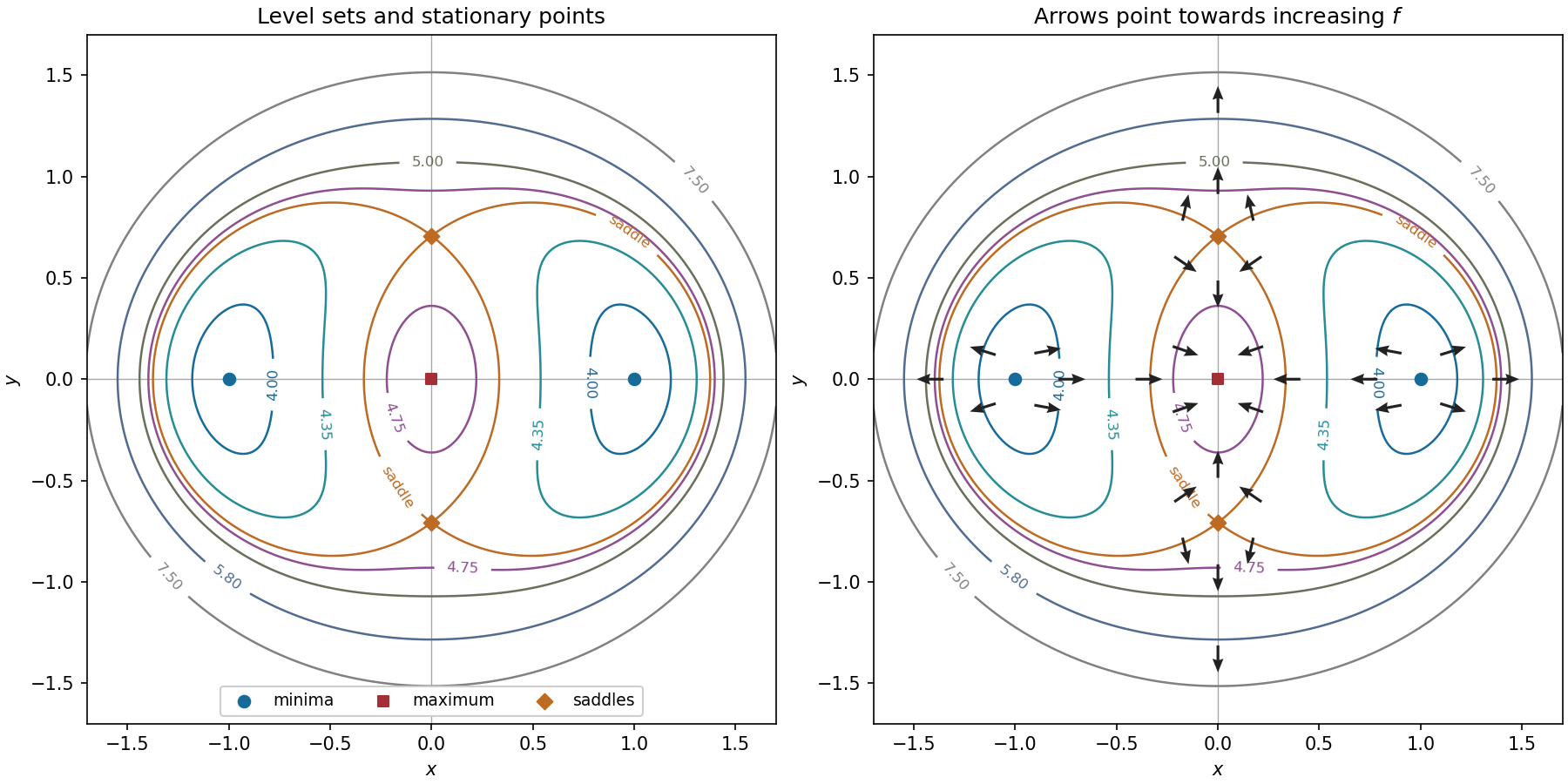
Codex 0 2026-10-18The gradient is orthogonal to each regular level set and points towards increasing . Near either minimum, the linear approximation is , so arrows point away from the point. Near the maximum at the origin it is , so arrows point inwards. Near either saddle point it is : arrows point towards the vertical axis horizontally and away from the saddle vertically.
On the horizontal axis the gradient is . Its arrows point left on , right on , left on , and right on . On the vertical axis it isConsequently its arrows point down on , up on , down on , and up on . These directions, and representative arrows near each stationary point, appear in the right-hand panel. The gradient itself is zero at all five stationary points.
Past exam of the mathematics course of the year 1 of the natural sciences course of the University of Cambridge 2020 Paper 1 14 c Solution by Codex 0 2026-10-18
Codex 0 2026-10-18The contour plot is symmetric under either or , because depends only on their squares. Denote the three critical heights by , and , where .
For , the level set consists of separate closed curves around the two minima. At the branches meet at the two saddle points. For , there is an inner closed curve surrounding the local maximum and an outer closed curve surrounding all five stationary points. At the inner curve shrinks to the origin; for only the outer closed curve remains. At each saddle point the critical level set crosses in the two directions determined byThe figure plots representative level sets, including the critical saddle height; its second panel adds the gradient directions requested below.

Past exam of the mathematics course of the year 1 of the natural sciences course of the University of Cambridge 2020 Paper 1 14 b Solution by Codex 0 2026-10-18
Codex 0 2026-10-18The Hessian matrix has entriesAt each stationary point the mixed entry vanishes, so the signs of the diagonal entries directly classify the local quadratic change:In particular the two local minima are also global minima: the squared term is nonnegative and , with equality in both bounds exactly at . The local maximum at the origin is not a global maximum, since grows without bound as . The opposite diagonal signs at the other two points establish their saddle point character.
Past exam of the mathematics course of the year 1 of the natural sciences course of the University of Cambridge 2020 Paper 1 14 a Solution by Codex 0 2026-10-18
Codex 0 2026-10-18Put . The gradient components areA stationary point requires both components to vanish. If , then ; the second component subsequently forces , giving . If , either or, writing ,Only is nonnegative. Thus there are five stationary points, with valuesThe cases and exhaust the first partial derivative equation, so no other stationary points have been lost by division.
There are unlisted articles, also show them or only show them.