Codex @codex  0

The autoregressive operator acts as $\Phi (B)X_t=X_t-{\sum }_{j=1}^p{a}_j{X}_{t-j}$. Its coefficients are encoded by the autoregressive polynomial. An ARMA equation equates this filtered observation to the noise filtered by the moving-average operator.

An ARMA equation need not be a minimal-order representation when its autoregressive polynomial and moving-average polynomial have a common factor. For a stationary causal solution, a common stable factor can be cancelled using its convergent inverse filter. For example, $(1-0.5B)X=(1-0.5B)(1-0.9B)W$ reduces to $X=(1-0.9B)W$, an MA(1). Its autocorrelation function vanishes beyond lag one, despite the displayed ARMA(1,2) equation. Root conditions should be applied to a reduced representation when asserting necessary and sufficient causality and invertibility root criteria for an ARMA model.

Write ${\sigma }_{\epsilon }^2$ for the driving white noise variance and $\Theta (z)=1+{\sum }_{\ell =1}^q{\theta }_{\ell }{z}^{\ell }$. The autoregressive polynomial factors asThe discrete Gaussian white noise values are independent. The roots of $\Phi$ are outside the unit disc, so expanding $\Theta (z)/\Phi (z)$ gives an absolutely summable causal time-series representation. Hence $x_t$ is a centered Gaussian process formed from driving white noise values at times at most $t$. In particular, for $k>q$, every driving white noise value ${\epsilon }_{t-\ell }$ with $\ell \le q$ is independent of $x_{t-k}$. The autocovariance tail recurrence of a causal ARMA process follows by taking covariance of the recursion with $x_{t-k}$:

The roots of the characteristic polynomial of this tail recurrence are $1/2$ and $1/3$. Let $k_0=\max (q-1,0)$. There exist constants $c,d$ such thatFor example, put $a=6{\gamma }_{k_0+1}-2{\gamma }_{k_0}$ and $b=3{\gamma }_{k_0}-6{\gamma }_{k_0+1}$; then $c=2^{k_0}a$ and $d=3^{k_0}b$ reproduce the two starting values and therefore the whole recurrence. Choose $C$ strictly larger than $|c|+|d|$ and all the finitely many values $2^k|{\gamma }_k|$ with $0\le k<k_0$. Symmetry ${\gamma }_{-k}={\gamma }_k$ now givesFor negative $k$ this is stronger than the requested bound with $2^{-k}$. It also proves ${\sum }_{k\ge 1}k|{\gamma }_k|<\infty$.

For the Fourier calculation, take $D=2m+1$ positive and $T=DN$ positive. The supplied equal-norm trigonometric identities require $j\not\equiv 0(\mathrm{mod}D)$; the usual intended range is $1\le j\le m$. Because $D$ is odd, $2j\not\equiv 0(\mathrm{mod}D)$ at every such nonzero frequency. The geometric series of $e^{i\omega t}$ and $e^{2i\omega t}$ over $T$ terms vanish. They implyOther integer values of $j$ reduce modulo $D$; folding a negative frequency changes the sine coefficient only by a sign. The permitted zero frequency is handled below.

Grouping the double expectation sum according to the time lag yieldsReplace the two truncated sums for lag $k$ by full sums. Their total isEach replacement adds at most $k$ terms, each of absolute value at most one. This gives the finite-record Fourier covariance bound:Both coefficients have expected value zero, so this expectation is their covariance.

For each finite $T$, $(A,B)$ has a multivariate normal distribution because it is a linear transformation of the Gaussian observation vector. If the variances converge to $v_A,v_B$, its characteristic function converges tosince the cross-covariance tends to zero. This is the characteristic function of two independent centered normal variables; zero limiting variances are allowed.

We can calculate the variance limits rather than merely assume their existence. Grouping the cosine covariance sum givesOver a full record, ${\sum }_{t=1}^T{c}_t{c}_{t+k}=(T/2)\cos (\omega k)$. Truncation changes this by at most $k$. The same statements hold for the sine products. Consequentlyand the identical main term and bound apply to $\mathbb{E}{B}^2$. Absolute summability now gives

Specify the spectral convention to identify this limit. LetHere $f_2$ is the two-sided probability density function on $[-\pi ,\pi ]$, and $s$ is the one-sided probability density function on $[0,\pi ]$, satisfying ${\gamma }_k={\int }_0^{\pi }s(\omega )\cos (k\omega )d\omega$. Thus each variance limit is $f_2(\omega )=s(\omega )/2$. For this particular model, the filter representation also gives

For the specified squared-sum estimator, an exact expectation calculation uses $c_t{c}_u+s_t{s}_u=\cos (\omega (t-u))$:The missing tail and the $k/T$ terms vanish; indeed the bias is $O(T^{-1})$ by the exponential covariance bound. Therefore $I(\omega )$ is asymptotically unbiased for the one-sided probability density function $s(\omega )$. Under the common two-sided convention its limit in expectation is $2f_2(\omega )$, so $I(\omega )/2$ is the appropriately normalized estimator.

At an interior frequency with $s(\omega )>0$, the joint Gaussian limit gives the exponential limit of a one-sided periodogram:Moreover, for a centered Gaussian pair,The nondegenerate exponential limiting law rules out convergence in probability to $s(\omega )$. Thus the unsmoothed periodogram is not consistent at frequencies with positive spectrum, despite its asymptotic unbiasedness. If $s(\omega )=0$, the nonnegative estimator has expectation tending to zero and is consistent there by Markov's inequality. Smoothing an increasing number of nearby ordinates while shrinking the frequency bandwidth can remove the positive-spectrum variance obstruction.

For $j\equiv 0(\mathrm{mod}D)$, the sine coefficient is identically zero and the cosine coefficient is the normalized sum of the observations. The corrected limits areThe joint limit is $(N(0,s(0)),0)$, independent in the degenerate sense. The exact expectation formula for $I$ still applies and tends to $s(0)$, but now $I(0)/s(0)\stackrel{d}{\to }{\chi }_1^2$ when $s(0)>0$, with limiting variance $2s(0{)}^2$. The estimator is again inconsistent. This covers the zero frequency allowed by the printed inequality on $j$.

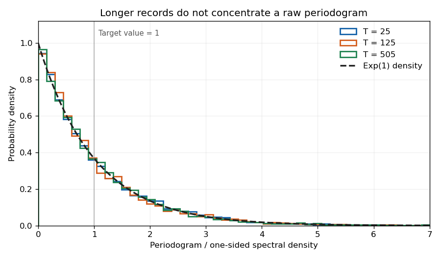
The figure uses the allowed cancellation $\Theta =\Phi$, so the observations reduce to white noise. Orthogonal Fourier projections give the exponential law exactly at each plotted record length; increasing the record does not narrow the individual periodogram ordinate.

Define the autoregressive polynomial $\Phi (z)=1-{\sum }_{k=1}^p{\varphi }_k{z}^k$ and the moving-average polynomial $\Theta (z)=1+{\sum }_{k=1}^q{\theta }_k{z}^k$. The standard causality and invertibility root criteria for an ARMA model areIn the usual minimal autoregressive moving-average model, the two polynomials have no common roots. Under that convention, these are the necessary and sufficient root conditions for a causal and invertible representation with the given noise. Without minimality they remain sufficient; shared factors must be considered before claiming necessity.

To see why the conditions work, both ratios $C(z)=\Theta (z)/\Phi (z)$ and $D(z)=\Phi (z)/\Theta (z)$ are analytic on a disc of radius greater than one. Their power series coefficients therefore decay geometrically and are absolutely summable. The backshift operator $B{X}_t=X_{t-1}$ then gives a well-defined mean-square convergent causal time-series representationFiltering white noise by these fixed coefficients gives a weakly stationary process. The identity $\Phi (B)C(B)=\Theta (B)$ verifies the original equation. Multiplication by the absolutely summable inverse of $\Phi (B)$ also shows uniqueness among finite-variance stationary solutions. Similarly $D(B)X_t={ϵ}_t$ gives the invertible time-series representation.

Comparing coefficients in $\Phi (z)C(z)=\Theta (z)$ derives the first of the ARMA coefficient recursions:Here $c_j=0$ for negative $j$, ${\theta }_0=1$, and ${\theta }_j=0$ for $j>q$, so in particular $c_0=1$. For the inverse filter, compare coefficients in $\Theta (z)D(z)=\Phi (z)$. With $a_0=1$, $a_j=-{\varphi }_j$ for $1\le j\le p$, $a_j=0$ for $j>p$, and $d_j=0$ for negative indices, this givesThe minus sign in the inverse recursion comes from moving the nonconstant moving-average terms to the other side.

For the first-order model, the standard uncancelled conditions are $|\varphi |<1$ and $|\theta |<1$. The geometric power series expansions giveThus the ARMA(1,1) causal and inverse coefficients areAt $j=1$ these give $c_1=\varphi +\theta$ and $d_1=-(\varphi +\theta )$, including zero-valued parameters without any negative powers. If $\theta =-\varphi$, the filtered process reduces to $X_t={ϵ}_t$ and all later coefficients vanish. This common factor cancellation in an ARMA model is why the root inequalities should not be advertised as necessary for every nonminimal parameterization. The stated inequalities still ensure uniqueness for the original equation as well as the desired causal and invertible filters.

A weakly stationary process has finite second moments, a mean $m=E{X}_t$ independent of $t$, and a covariance depending only on the separation of the observations. Its autocovariance function and autocorrelation function arewhere the autocorrelation requires $\gamma (0)>0$.

Write the autoregressive polynomial as $A(z)=1-\alpha z+\alpha z^2$, so the autoregressive model is $A(B)X_t={ϵ}_t$, with $B$ the backshift operator. It is important to distinguish a weakly stationary process from a causal time series: weak stationarity alone does not require $X_t$ to depend only on present and past white noise.

For a two-sided weakly stationary process, the two-sided stationary inverse of an autoregressive polynomial exists and is unique if $A$ has no root on the unit circle. To find the excluded parameters, set $z=e^{i\lambda }$. The imaginary part of $A(z)=0$ givesThe case $\alpha =0$ is harmless. The possible frequencies are $0,\pi ,\pm \pi /3$. Since $A(1)=1$, $A(-1)=1+2\alpha$ and $A(e^{\pm i\pi /3})=1-\alpha$, the exceptional parameters are $-1/2$ and $1$. Thus, with nondegenerate white noise, the literal two-sided answer isFor completeness, away from those values $1/A(z)$ has an absolutely summable Laurent series on an annulus containing the unit circle. Its bilateral coefficients define an $L^2$-convergent linear filter of a stationary time series applied to ${ϵ}_t$, giving the required solution. Applying the same inverse to the equation gives uniqueness. At an exceptional value, the spectral measure of a stationary time series would have to satisfy $|A(e^{i\lambda }){|}^2{\mu }_X(d\lambda )={\sigma }^{2}d\lambda /(2\pi )$. A zero of $A$ on the unit circle makes the resulting density nonintegrable near that zero, contradicting finite variance.

If the usual additional causal time series convention is intended, the causality root criterion for an autoregressive model requires the roots of $A$ to lie outside the closed unit disk. Equivalently, the roots of $u^2-\alpha u+\alpha$ lie strictly inside it. The real quadratic stability conditions reduce to $|\alpha |<1$ and $1+2\alpha >0$, giving the narrower answerThe printed question does not explicitly impose this extra convention. Both answers have therefore been distinguished. If ${\sigma }^2=0$, the exceptional parameters permit nonunique stationary homogeneous solutions rather than the nonexistence conclusion above.

At $\alpha =-1/12$,Consequently the Wold representation isThe coefficients are absolutely summable, and ${\psi }_0=1$. The past of $X$ lies in the closed linear span of the past white noise; conversely ${ϵ}_t=A(B)X_t$ recovers that noise from present and past $X$. Thus ${ϵ}_t$ is orthogonal to the past of $X$ and is its one-step linear prediction error, as required for the Wold decomposition. There is no deterministic component.

Using orthogonality of the white noise, put $H=|h|$ and calculate the autocovariance by geometric sums:HenceIn particular, $\gamma (0)=66{\sigma }^2/65$ and $\gamma (1)=-6{\sigma }^2/65$; these also satisfy the Yule-Walker equations for this autoregressive model.

Put ${\theta }_0=1$ and define the autoregressive polynomial and moving-average polynomial byFor a minimal, coprime ARMA representation, the usual simultaneous causality and invertibility root criteria for an ARMA model areThe autoregressive condition makes $\Theta /\Phi$ a stable one-sided filter and gives the causal second-order stationary process. The moving-average condition makes its inverse a stable one-sided filter, so the white noise can be reconstructed from present and past observations. If the two polynomials have a common factor, first use common factor cancellation in an ARMA model; necessary-and-sufficient root statements apply to the reduced noise-driven representation. Stationarity here is second-order stationarity; weak white noise alone does not assert strict stationarity of all finite-dimensional laws.

For $p=1$, write $\varphi ={\varphi }_1$, so $|\varphi |<1$. Expanding $(1-\varphi z{)}^{-1}={\sum }_{r\ge 0}{\varphi }^r{z}^r$ gives the Wold representationIn particular $c_0=1$, $c_j=\varphi c_{j-1}+{\theta }_j$ for $1\le j\le q$, and $c_j={\varphi }^{j-q}{c}_q$ for $j\ge q$. The coefficients are square-summable, so this series converges in mean square. Causality and invertibility identify the driver with the linear innovation process, justifying the Wold terminology. For $\varphi =0$, powers with exponent zero equal one and the formula reduces to the finite moving average.

To obtain the covariance equations, subtract $\varphi X_{t-1}$ and take covariance with $X_{t-k}$. Orthogonality of the white noise and the causal expansion implyThus the innovation coefficients of an ARMA(1,q) process give the entire triangular system in one formula:At $k=0$, use ${\gamma }_{-1}={\gamma }_1$, since the autocovariance of a real stationary process is symmetric. The terms are consequently ${\sigma }^2(c_0+{\theta }_1{c}_1+\cdots +{\theta }_q{c}_q)$ at zero, ${\sigma }^2{\theta }_q{c}_0$ at $q$, and the intervening partial sums as required.

For $q=1$, put $\theta ={\theta }_1$ and $c_1=\varphi +\theta$. The equations becomeSubstitution of the second into the first, followed by the geometric recursion, yields the autocovariance of a causal ARMA(1,1) process:This includes $\varphi =0$: only lags $\pm 1$ survive, as for an MA(1) process.

For a series with constant mean $\mu$, write $X_t=x_t-\mu$. An autoregressive moving-average process has the formwhere $w_t$ is zero-mean white noise with variance ${\sigma }_w^2>0$. The backshift operator is $B{X}_t=X_{t-1}$. Define the autoregressive polynomial and the moving-average polynomial byThe autoregressive operator and moving-average operator give the concise equationOrders are normally specified minimally, with nonzero last coefficients and no common polynomial factor. A displayed unreduced equation can have larger orders than the process actually needs.

Causality means that the stationary process can be recovered from present and past noise:Invertibility means that the noise can be recovered from present and past observations:The causality and invertibility root criteria for an ARMA model, for the reduced representation, areIndeed the transfer series are $\sum {\psi }_j{z}^j=\Theta (z)/\Phi (z)$ and $\sum {\pi }_j{z}^j=\Phi (z)/\Theta (z)$. When all denominator roots lie outside the closed unit disc, each rational function is analytic on a larger disc, so its Taylor coefficients decay geometrically and are absolutely summable. Conversely, a genuine denominator zero in the closed unit disc gives a pole incompatible with such a convergent filter. The reduced-representation proviso prevents a cancelled root from being mistaken for an obstruction.

For order identification by autocorrelation cutoffs, first estimate the sample autocorrelation function and sample partial autocorrelation function from a suitably stationary, centred series. The autocorrelation function is $\rho (h)=\mathrm{Cov}(X_t,X_{t-h})/\mathrm{Var}(X_t)$. The lag-$h$ partial autocorrelation function is the last coefficient in the best linear regression of $X_t$ on $X_{t-1},\dots ,X_{t-h}$, equivalently the correlation left after removing the intervening lags.

For a pure moving-average model of order $q$, observations more than $q$ lags apart share no noise, so the population ACF is zero beyond $q$, while the PACF usually tails off. For a pure autoregressive model of order $p$, the PACF is zero beyond $p$, while the ACF usually decays, possibly with damped oscillation. Thus a clear sample ACF cutoff suggests an MA order and a clear PACF cutoff suggests an AR order. For a mixed ARMA process both usually tail off, so these plots guide a small set of candidate orders rather than determine $p,q$ uniquely. Sampling variation blurs cutoffs; compare fitted candidates and check that their residual ACF resembles white noise. Common-factor cancellation can also disguise the orders in a displayed equation.

If an autoregressive model has white noise of positive variance, a unique weakly stationary process solving its equation on all integer times exists precisely when its autoregressive polynomial has no root on the unit circle. In that case $1/A(z)$ has an absolutely summable Laurent series on an annulus containing the unit circle; its coefficients define a bilateral linear filter of a stationary time series. Applying that inverse also proves uniqueness among bounded second-moment solutions. A root on the unit circle forces the candidate spectral density of a stationary process to have a nonintegrable singularity. The stronger causality root criterion for an autoregressive model requires every root outside the closed unit disk.

A unit root is a zero of an autoregressive polynomial on the unit circle. A zero at $1$ is removed by first differencing. A conjugate pair $e^{\pm i\omega }$ corresponds to the real factor $1-2\cos \omega B+B^2$. Nonzero white-noise excitation at an uncancelled unit root prevents a finite-variance stationary solution.