Codex @codex  0

A biconnected component is a maximal connected subgraph with no cut vertex of its own. We use the block convention that also includes each bridge in a graph with its two endpoint vertices, and each isolated vertex, as a biconnected component. A biconnected component with at least three vertices stays connected after any single vertex deletion. Distinct biconnected components share at most one vertex; the vertices belonging to more than one biconnected component are exactly the cut vertices. The shared-$A$ example has two biconnected components, its two triangles in a graph. The joined-$CD$ example has three: $ABC$, the bridge in a graph $CD$ with its endpoints, and $DEF$. The edges partition into these pieces, while the shared cut vertices occur in several pieces. ^[ref]

A cut vertex, also called an articulation point, is a vertex $v$ of an undirected graph whose deletion increases the number of connected components of a graph. Write $k(G)$ for that count, including isolated vertices, and $G-v$ for the graph obtained by removing $v$ and every incident edge. Then the test is $k(G-v)>k(G)$, even when the original graph is disconnected. By contrast, deleting a bridge in a graph removes just one edge and keeps both endpoint vertices. These are different failure models. ^[ref]

First take two triangles in a graph, $ABC$ and $ADE$, sharing only the vertex $A$. This simple graph hasHere $XY$ abbreviates the unordered pair $\{X,Y\}$. Removing $A$ leaves the two connected components of a graph $\{B,C\}$ and $\{D,E\}$, so $k(G-A)=2>1=k(G)$. Removing any other vertex leaves a connected graph. Thus $A$ is the only cut vertex. Every edge lies on a triangle in a graph, so deleting any single edge still leaves a graph path between its endpoints along the other two edges. There are no bridges in a graph.

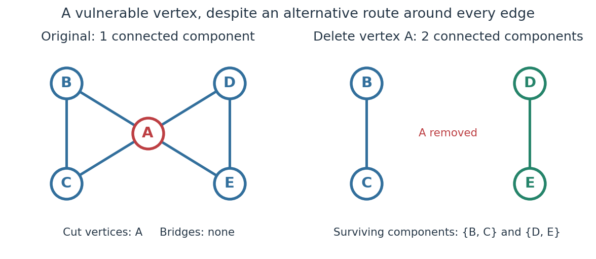
The generator computes the adjacency lists and checks every vertex deletion, giving the following complete table:

Now take two disjoint triangles in a graph, $ABC$ and $DEF$, joined by the edge $CD$:Deleting only $CD$ preserves all six vertices and leaves connected components of a graph $\{A,B,C\}$ and $\{D,E,F\}$: $CD$ is the only bridge in a graph. Deleting $C$ also removes $AC$ and $BC$, leaving connected components of a graph $\{A,B\}$ and $\{D,E,F\}$. Deleting $D$ instead leaves $\{A,B,C\}$ and $\{E,F\}$. Thus $C,D$ are exactly the cut vertices.

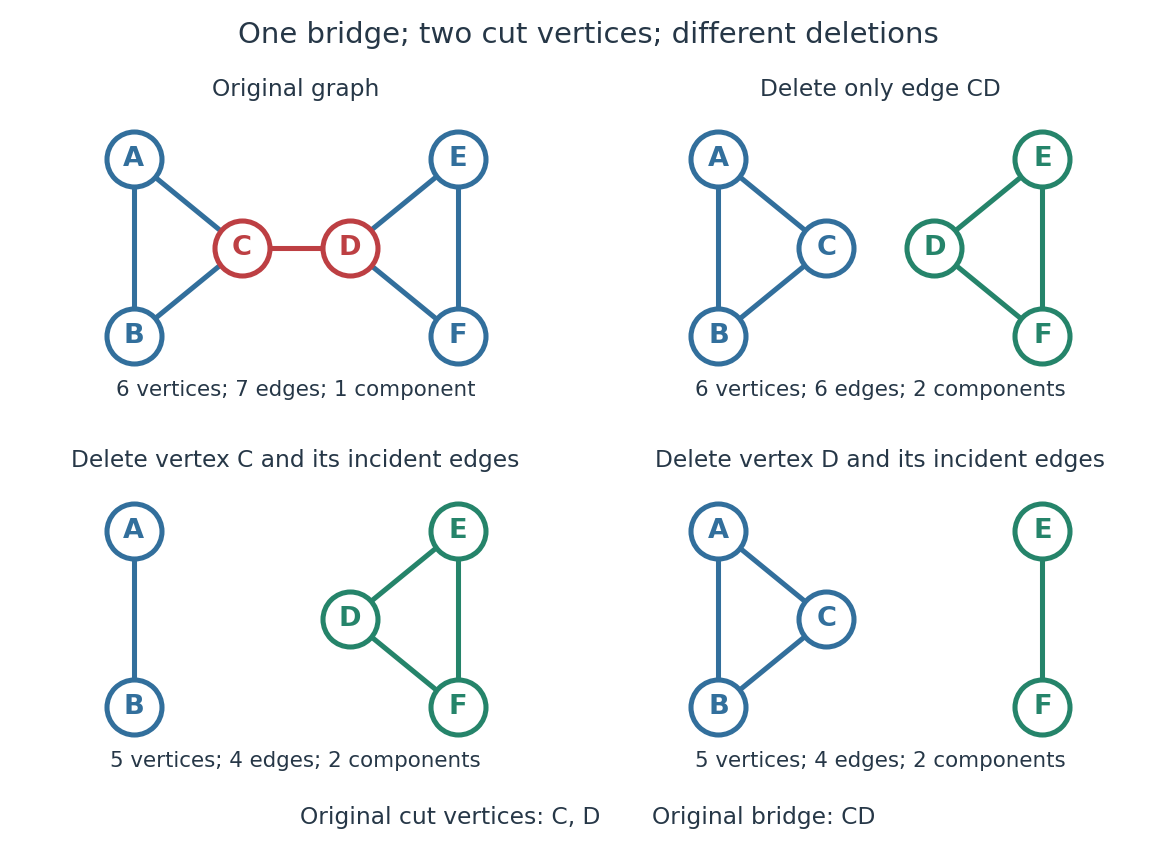
Again the adjacency lists and all vertex deletion counts are computed directly:

For a disconnected example, adjoin an isolated vertex $Z$ to the first graph. Now $k(G)=2$, deleting $A$ gives $k(G-A)=3$, and deleting $Z$ gives $k(G-Z)=1$. The original graph was already disconnected, but $A$ is still a cut vertex; $Z$ is not. The empty graph has count zero, so deleting the only vertex of a one-vertex graph does not create a cut vertex. Nor is either endpoint of a single isolated edge a cut vertex, although that edge is a bridge in a graph.

In a communications network, a cut vertex models a router whose failure separates surviving routers. The shared-$A$ example shows why having an alternative graph path around each individual edge does not protect against failure of the common router. An additional edge from $B$ to $D$ removes this particular vulnerability: after deleting $A$, $B,D$ still join the two sides. A bridge in a graph instead models a vulnerable link. This distinction tells us whether to add another cable between existing devices or a route avoiding an indispensable device; it describes connectivity, rather than traffic capacity or failure probabilities.

The beautiful structural consequence is that a graph splits into biconnected components joined at cut vertices. Within each nontrivial robust piece, a single vertex failure cannot separate the other vertices; between pieces, the shared cut vertices reveal the bottlenecks. Also, a Hamiltonian graph has no cut vertex: deleting any vertex from its Hamilton cycle leaves a Hamiltonian path through all remaining vertices.

Historically, Tarjan's June 1972 paper developed depth-first search as a tool for finding biconnected components in time linear in the numbers of vertices and edges. ^[ref] In his 1983 recollection, Tarjan credited Hopcroft with the original linear-time biconnected component algorithm during their collaboration beginning in summer 1970, and described the published version as a refinement. The historical lesson is how a carefully organized traversal turns many separate deletion experiments into one computation. ^[ref]