Here "finite" refers to the description: a short algorithm can perform arbitrarily many steps on increasingly large inputs. Solving a computational problem additionally requires termination and the specified output on every permitted input. State assumptions explicitly: binary search requires a sorted array.
An algorithm is an idea that can have implementations in different programming languages. Its explanation should make three things visible: the permitted inputs, the rule for each step, and the meaning of the returned output. Algorithm correctness then separates finding the right answer from eventually finishing; time complexity asks how much work finishing requires.
A particularly useful design question is: what knowledge survives each step? In binary search, it is the location of every possible match inside the remaining candidate range. Writing that fact as a loop invariant turns an intuitive shortcut into a procedure whose discarded candidates can be justified. This often helps discover the algorithm, rather than merely check it afterward.
Given a fixed sequence of compatible matrices , choose a binary parenthesization of that minimizes the number of scalar multiplications in ordinary matrix multiplication. The order of the matrices is fixed: parenthesization changes the grouping, not the operand order. Associativity preserves the product while intermediate matrix dimensions change the cost. The possible binary groupings are counted by the Catalan number for .
A greedy algorithm commits to a locally preferred next choice without revisiting earlier choices. Its rule needs a justification to guarantee a globally optimal result: the largest-individual-value rule in the 0-1 knapsack problem example fails, whereas Dijkstra's algorithm correctly settles the smallest tentative distance under its nonnegative-edge assumptions.
Partial correctness means that, if the algorithm terminates on a permitted input, its output meets the specification. Total correctness additionally requires termination on every permitted input.
Establishing specified properties of a system using formal proofs about a precise model. Formal verification connects an implementation to a formal specification; correctness of the model and its assumptions still matters when applying the result to a physical system.
A mathematically precise description of permitted behaviour. A formal specification for the microkernel file-read example's service could relate an authorized request to the exact returned bytes; a formal specification of its microkernel's IPC need only describe the protected transport operation. They state different obligations.
Conformance of compiled machine code to the behaviour of the code model used to justify it. Binary correctness can extend formal verification across the compilation step; the result applies to the particular compiled artifact and its assumptions.
Conformance of an implementation's behaviour to its specified functional requirements. The exact obligations come from the formal specification: correct delivery of an IPC payload and correct computation of a file read are different requirements. Neither requirement by itself supplies a numerical response-time bound.
A statement true whenever execution reaches a chosen point in a loop, usually immediately before its condition is tested. Establish it initially, preserve it through each iteration, and combine it with the exit condition to establish algorithm correctness. Termination needs a separate argument.[ref]
Linear search, also called sequential search, examines a finite sequence from its beginning, performing an equality test on each entry until one matches the target or the entries run out. It needs no sorted array or total order on the values. This makes it useful for a small collection, a one-off lookup, or data available only in succession: the next entry is enough to make progress.
Specify the answer precisely. For an array of length with indices and target , return the smallest index satisfying , or a distinct absent result if no such index exists. Repeated values are allowed. In this contract, finding a later duplicate is insufficient when an earlier match exists. Assume the input remains unchanged during the search and each equality test terminates with a stable truth value expressing the intended matching relation.
Here is an implementation in Python; The official Python sequence method
None represents absence and is distinct from the valid index zero:def linear_search(entries, target):
for index, entry in enumerate(entries):
if entry == target:
return index
return Nones.index(x) likewise specifies the first occurrence, but signals absence by raising ValueError. An API's absent-result convention belongs to its contract.[ref]Take the original unsorted array . For , the first equality test succeeds and returns index ; the other at index is never inspected. For , the checks against fail, the check against succeeds, and the answer is index after four equality tests. For absent target , all five equality tests fail and the answer is
None. On the empty sequence, there is no entry to inspect: return None with zero equality tests.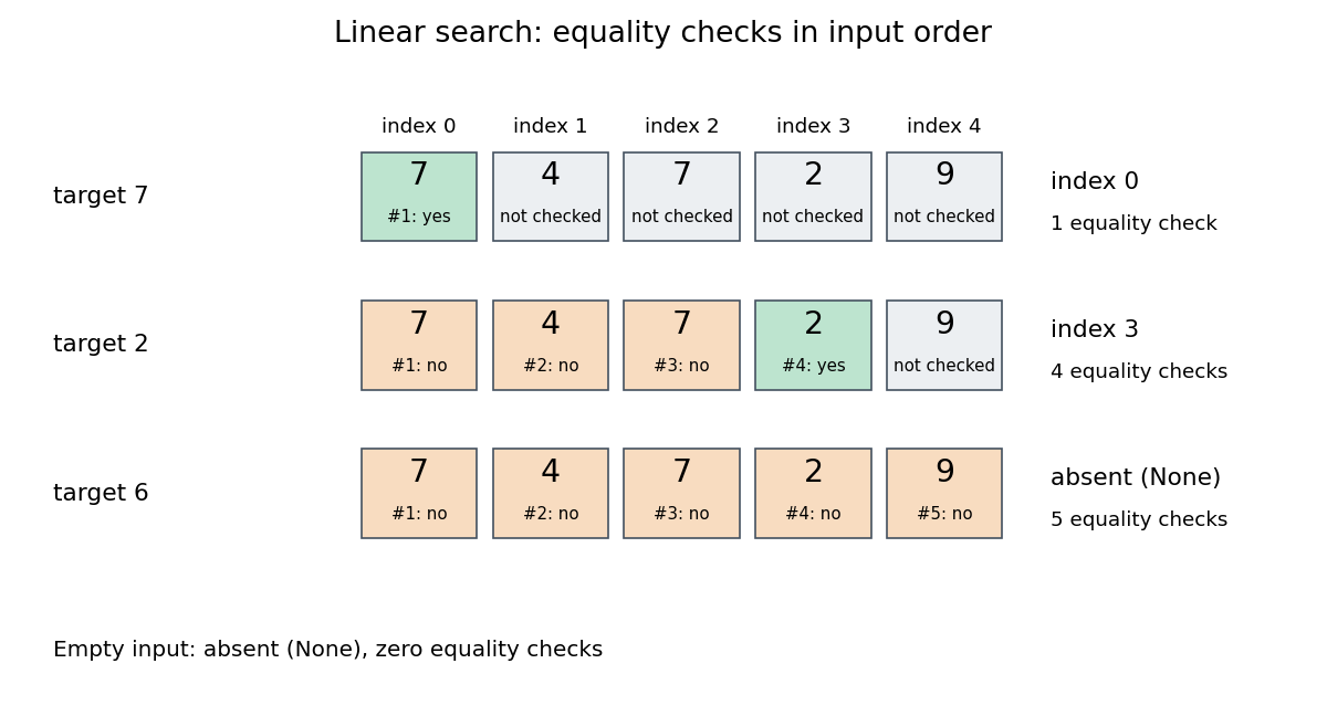
Value order never justifies skipping an entry in this algorithm. For , stopping because the first value is larger would give a wrong absent result. Any permutation of the input remains searchable by linear search, although the first matching index and number of equality tests can change. By contrast, binary search uses a total order and the sorted array property to discard whole candidate ranges. Its logarithmic time complexity additionally assumes cheap access to middle entries; a sorted linked list does not acquire constant-cost indexed access merely by being sorted. Sorting for a single query also has a cost, and changes positions relative to the original sequence.
Count just the equality tests between the target and an entry, excluding loop conditions and index updates. If the first match is at index , linear search uses exactly equality tests. If the target is absent, it uses exactly . Thus for the best successful case costs one equality test, and the worst case costs , attained by absence or a first match at the last index. For , the sole outcome is absence with .
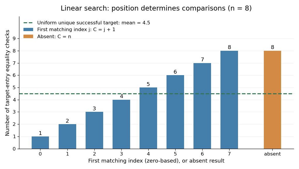
An expected value needs a specified probability distribution. For , condition on success, assume the target occurs exactly once, and assume its position has a uniform distribution on a finite set of indices . Then the expected value of the linear search comparison count isThis is the average of the costs under those assumptions, with no assumption that the array is sorted. It is not a universal average for arbitrary queries. For example, with , a unique successful target at index with probability and at index with probability has expected value , rather than .
Duplicates also require care about what is sampled. Choose a position uniformly in , then search for its value. All queries succeed, but the five possible sampled positions give costs : both positions holding cause an immediate match at index . The expected value is , not . Uniformly choosing an occurrence does not uniformly locate the first match.
More generally, let the success probability be and let be the conditional probability that the first matching index is , allowing duplicates. Since , the expected value isUnder the unique, uniformly located successful-target assumptions this becomes . If every query is absent, and without needing conditional probabilities. When , success is impossible and ; the successful-search conditional formula is undefined.
Converting the linear search comparison count to execution time needs a cost model. Under constant-cost equality tests, next-entry access, and loop bookkeeping, worst-case time complexity is in Big O notation for , with constant overhead even for the empty sequence. Variable-length entries can make an equality test expensive. On a linked list, advance along its links; repeatedly restarting at the head to obtain the next numeric index adds work that the comparison count does not capture. These are exact operation counts and conditional mathematical averages, not runtime measurements.
The loop invariant just before inspecting index is: , and no entry at an index matches . Initially , so there are no earlier entries. A failed equality test extends the excluded region by one position and preserves the loop invariant. A successful equality test at index establishes a match; the loop invariant establishes that it is the first one. At exhaustion, and every entry has failed, so the absent result is correct. The number of remaining entries decreases after each failed equality test, proving termination for a finite sequence. Together these establish algorithm correctness under the assumptions that the input is stable and each equality test terminates. No step of the argument compares the relative order of values.
A terminating check returning whether two values match under a specified relation. Mathematical equality is one such relation; a chosen equivalence relation can instead express matching keys. Linear search only needs this check, whereas binary search also uses relative order. The cost of an equality test depends on the representation and implementation of its operands.
Replace an operation by an equivalent operation sequence with lower cost on the target machine. For fixed-width wrapping integers, multiplication by eight equals left shift by three, and multiplication by fifteen equals left shift by four minus the original operand. Condition codes and wider results must also be preserved if the original machine instruction exposes them.
// Destination: computer-science.bigb
Periodically sample an executing program's instruction pointer and accumulate an address histogram. Samples approximate time spent in address regions, rather than exact instruction execution counts. Jittering the sampling interval reduces accidental synchronization with periodic code.
// Destination: computer-science.bigb
Depth-first search is a graph search that follows a branch as far as it can before returning to try the next unexplored branch. Starting at a vertex of an undirected graph on a finite set of vertices, mark as discovered. Scan its graph neighbours in a fixed order: for each undiscovered vertex, record the current vertex as its parent in a rooted tree in the discovery tree, mark the new vertex, and explore it immediately using recursion. Return when its adjacency list is exhausted. Discovery marks persist after return, preventing a graph cycle from causing repeated exploration. This branch-and-return rule is the maze exploration described in MIT's notes. [ref]
Use the same unweighted undirected graph as breadth-first search, with vertex set and edgeswhere denotes the unordered pair . Visit graph neighbours in lexicographic order of their one-letter labels, starting at . The discovery order, computed by the diagram's generator, isThe discovery edges in order are . They form a rooted tree spanning the reached vertices, with root of a tree . The other edges, and , remain in the original graph but never discover a new vertex. In particular, the graph cycle causes no repeated discovery.
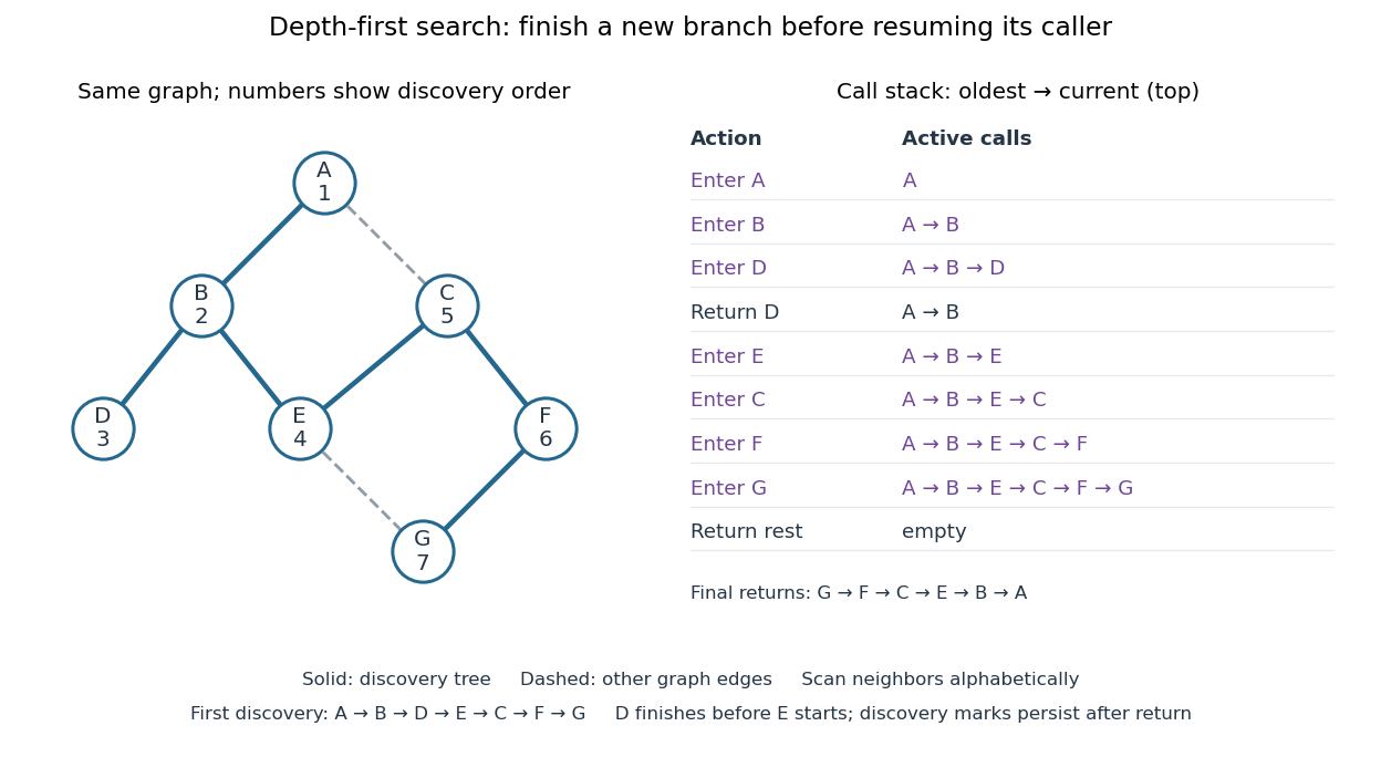
At there is no undiscovered graph neighbour, so its call returns to . The next call enters , then , then , then . Immediately after discovering , the call stack is , with on top; is still discovered but its call has finished. The maximum call stack depth is six, although seven vertices are discovered. Following the recorded parent in a rooted tree backwards at each step reconstructs a graph path; here the route from to is , using five edges. Breadth-first search instead finds , using three edges. Depth-first search establishes reachability but does not guarantee the fewest edges.
An explicit LIFO stack can replace recursion, but its entries and discovery rule must be specified. To reproduce this exact traversal, store one frame per active vertex, retaining the next position in its adjacency list. Advance the top frame by one graph neighbour; if that vertex is undiscovered, mark it and push its frame immediately; pop an exhausted frame. Pushing all undiscovered graph neighbours at once and marking them on push is a different iterative variant. Even pushing them in reverse lexicographic order does not generally reproduce the parent in a rooted tree relationships above: would already be marked while processing , so could not discover .
With an adjacency list representation, constant-cost discovery checks and frame operations, and the graph neighbours already ordered, depth-first search has time complexity in Big O notation. Each reached vertex is entered once and each incident edge is examined at most twice in an undirected graph; initializing all discovery marks costs . The call stack has depth at most , since no active vertex repeats. Discovery marks and the recorded parent in a rooted tree for each nonroot vertex also need auxiliary space complexity, excluding storage for the graph. Sorting adjacency lists to obtain a chosen order is additional work. [ref]
https://raw.githubusercontent.com/kevin-wayne/algs4/master/src/main/java/edu/princeton/cs/algs4/DepthFirstPaths.java. Sedgewick and Wayne, Algorithms: DepthFirstPaths discovery marks and resource bounds
One start explores only its connected component of a graph. To cover a disconnected graph, start again at every still-undiscovered vertex while keeping all discovery marks; the discovery trees form a forest. Depth-first search is useful for reachability, constructing a spanning tree of a connected graph, and organizing the return steps needed by a depth-first traversal of a tree. For detecting a graph cycle in a simple graph that is an undirected graph, an edge to an already discovered vertex other than the current parent in a rooted tree closes a graph cycle; the immediate return edge to that parent in a rooted tree is not itself a graph cycle.
// Target: computer-science.bigb
Memoization retains a completed function result under a memoization key and returns that result when an equivalent request recurs. For a terminating pure function, repeated evaluation can therefore become lookup rather than repeated work. The benefit is especially striking with recursion and overlapping subproblems: a large tree of calls can refer to a small Directed acyclic graph of distinct answers. The memoization cache contract determines whether reuse is correct; the memoization cache lifetime determines whether an answer is still present when wanted.
Memoization records computed answers, whereas a memory cache retains data from computer memory. A CPU cache hit does not by itself prevent a program from evaluating the same function again. Spreadsheet dependency evaluation adds an explicit mechanism for invalidating affected cached cell values after inputs change; a general memoization table does not discover such changes automatically.
A documented early motivation was to let programs improve their efficiency during execution through rote learning: the abstract of a 1968 paper explicitly proposes such a programming language facility.[ref]
“Memo” Functions and Machine Learning by Donald Michie. Donald Michie, “Memo” Functions and Machine Learning, Nature 218, pp. 19–22 (1968), abstract: programming-language rote learning motivated by efficiency during execution
Overlapping subproblems occur when several parts of a calculation request the same smaller problem. Memoization can share its answer if the memoization key identifies that problem completely. For the Fibonacci numbers, both and require . In dynamic programming, the dynamic programming state plays the corresponding role of identifying a reusable continuation. Overlap explains potential savings; the recurrence relation and its base cases still need to be correct.
The Fibonacci numbers give an exact example. For a nonnegative integer , their recurrence relation isTo obtain by direct recursion, evaluate and separately; computing also evaluates . The full call tree has 15 occurrences but just six distinct arguments, . Shared dependencies form a Directed acyclic graph because every directed edge goes to a strictly smaller argument. Memoization evaluates a distinct argument on first demand; filling values in increasing argument order is the corresponding bottom-up dynamic programming calculation.[ref]
Lecture 15: Recursive Algorithms (6.006 Spring 2020) by Massachusetts Institute of Technology, 6.006 course staff. MIT 6.006 Spring 2020, Lecture 15: Recursive Algorithms, printed pp. 2–3, Fibonacci Numbers and Re-using Subproblem Solutions
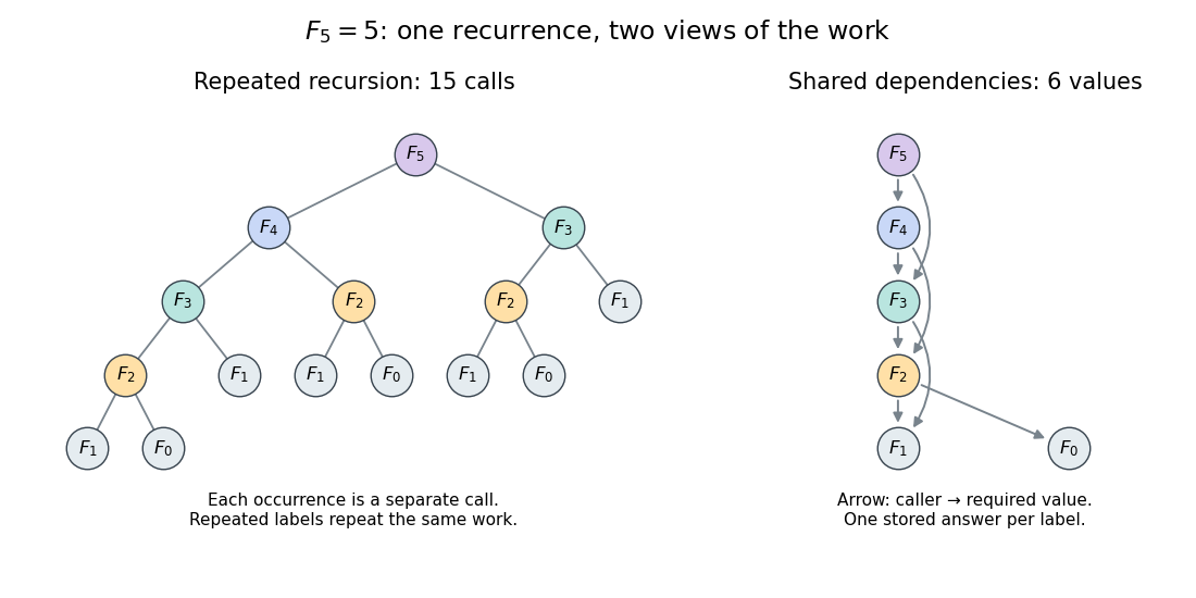
Repeated calls for Fibonacci numbers and their shared Directed acyclic graph of dependencies
. The call tree contains 15 occurrences for . The dependency graph contains six distinct arguments and eight directed edges. Equal labels have equal colors; arrows in the right panel point from a caller to the value it requires. Details.Use an initially empty hash table
memo, shared by every recursive call. Count even the first evaluations of the two base cases, store only completed results, evaluate the left term first, and retain all entries. The following original procedure assumes a nonnegative integer argument:def cached_fib(n, memo):
if n in memo:
return memo[n]
if n < 2:
value = n
else:
value = cached_fib(n - 1, memo) + cached_fib(n - 2, memo)
memo[n] = value
return valueEvery self-call must pass through the memoization lookup. Wrapping only the outer call while leaving inner calls uncached retains the repeated work. Test membership rather than whether the stored value is nonzero: is a valid completed result.
For cold , the lookup arguments are . The first six are absent; the last three reuse completed answers. Results are stored on return in argument order , with values . Thus there are nine wrapper calls, six body evaluations and four additions. Repeating with the same table takes one wrapper call and no body evaluation. Requesting next evaluates only its body, reuses and , and stores : three wrapper calls, one body evaluation and two hits.
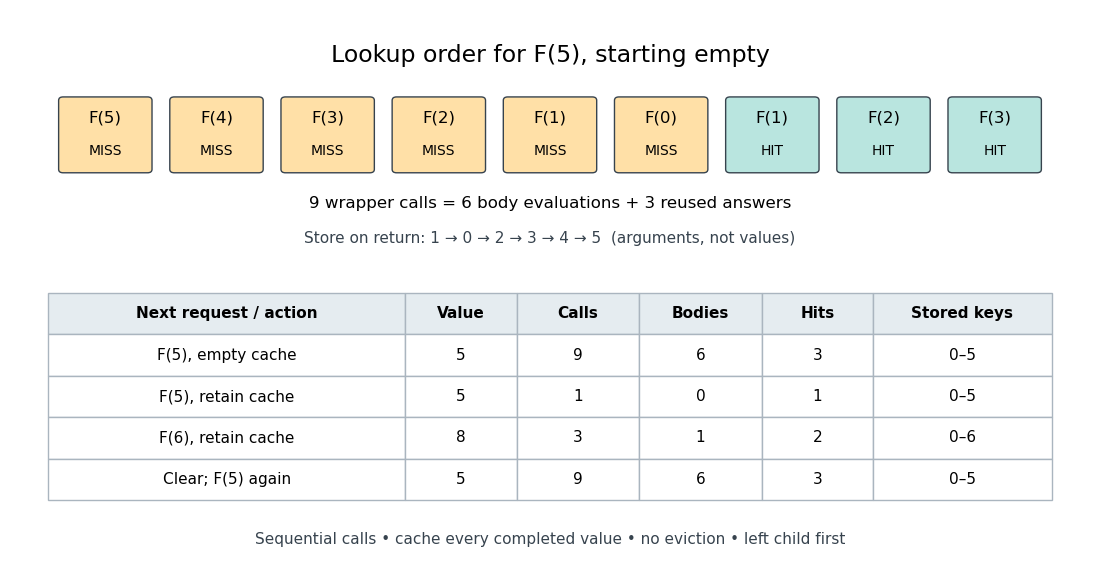
An exact memoization lookup trace and the effect of retaining or clearing its table
. The first row records cold lookup order. The table records successive requests with one retained table; clearing it before the final request restores the cold counts. Calls include lookups that immediately return stored values; bodies count only first evaluations. Details.The direct-call count satisfies and . Its exact solution is , as substitution into this recurrence relation verifies. With the specified memoization procedure, a cold call at evaluates distinct bodies, makes additions and makes wrapper calls. There are hits: each of the nonbase bodies issues two recursive calls, in addition to the initial call. The difference is between the number of occurrences and the number of distinct subproblems.
Under constant-cost lookup and integer addition, Memoized Fibonacci evaluation has time complexity in Big O notation, retaining values. A hash table needs its own lookup-cost assumptions; an array indexed by avoids hash collisions in this example. Memoization removes repeated bodies, but also pays for keys, lookups and retained answers. A workload without reuse can pay those costs without saving evaluations.
The call stack remains. Left-first recursion descends through arguments before returning, giving simultaneously active frames for . Therefore the auxiliary space complexity includes frames as well as table entries in the constant-size-value model. An iterative bottom-up dynamic programming calculation removes these recursive frames; retaining only the two previous Fibonacci numbers suffices when only the final value is wanted, but discards the table useful for later requests.
Exact Fibonacci numbers do not remain constant-size values. For , the recurrence relation gives , so the representation of as a binary number has order bits. With ordinary addition costing order bit operations on such operands, the additions cost order bit operations in total. Retaining all values also requires order bits of value storage, before keys and frame overhead. The linear bound counts additions under its stated cost model; it is not a linear bound on exact integer arithmetic in bits.[ref]
Lecture 15: Recursive Algorithms (6.006 Spring 2020) by Massachusetts Institute of Technology, 6.006 course staff. MIT 6.006 Spring 2020, Lecture 15: Recursive Algorithms, printed p. 3, final three bullets: growing Fibonacci bit lengths and addition cost
For a terminating pure function, a reusable entry must record its correct completed result, and equal memoization keys must imply equal results throughout the entry's memoization cache lifetime. Reusing that result must also preserve the behavior callers require. These conditions separate correctness from speed: a complete key can be correct even if it rarely repeats.
A procedure using deterministic computation can still have a required side effect. If a procedure returns and appends an audit record on every call, serving the second call from a table preserves the numerical answer but skips the second record. Likewise, if each call promises a fresh mutable list, returning the same stored mutable list changes observable sharing and allows a caller to damage later answers. Plain result reuse is unsuitable for those contracts.[ref]
functools — Higher-order functions and operations on callable objects (Python 3.14 documentation). Python documentation, functools.lru_cache: paragraph warning against functions with side effects, distinct mutable results, or impure time/random results
Completion matters for recursion. Suppose computing key needs key , and computing needs . A table containing only completed answers has no answer to return for the second ; remembering completed values does not make this directed cycle terminate. Marking a key
ACTIVE before descending detects re-entry, as in spreadsheet dependency evaluation, but detection is not a solution of the circular equations. If computation fails, clear its active mark and do not publish an unfinished value. The example using Fibonacci numbers avoids this issue through a strictly decreasing argument.The call counts above assume sequential execution and no eviction. Concurrent requests for an absent key can both begin evaluation before either publishes its result; keeping a table coherent alone does not ensure one body execution per key.[ref]
functools — Higher-order functions and operations on callable objects (Python 3.14 documentation). Python documentation, functools.cache and functools.lru_cache: thread-safe cache updates can still allow repeated evaluation before completion
A memoization key identifies all information that determines a reusable answer. Write for explicit arguments and for relevant context. For a function and key function , the necessary value condition isThis implication need hold only for contexts in which the entry can be reused. The condition concerns key equality, not merely equality of hash function outputs: a hash table must resolve hash collisions by comparing complete keys. Include the identity or version of the procedure if one table stores results for several procedures or changing implementations.
For an original toy example, let . Caching only by after incorrectly returns for , whose answer is . The pair is complete for this function. If is hidden in mutable configuration, either freeze that configuration for the memoization cache lifetime, include a reliable version in the key, or invalidate affected entries before reuse. A version is sufficient only if every relevant change updates it. Object identity alone is likewise insufficient for a mutable list whose contents determine the answer.
A memoization cache lifetime is the interval over which retained entries are available and valid. One table per top-level request shares recursive subproblems within that request; keeping a table between requests also allows the warm and incremental examples. Clearing it loses those savings. Evicting a correct answer can preserve correctness for a terminating pure function, while forcing recomputation; changing an input without invalidating an obsolete answer can break correctness.
Specify who owns the table, when context changes invalidate it, and how long keys and results occupy computer memory. In a concrete implementation, retained references can keep arguments and answers alive until removal or clearing.[ref]
functools — Higher-order functions and operations on callable objects (Python 3.14 documentation). Python documentation, functools.lru_cache: cache_clear and retention of argument and return-value references until eviction or clearing
The memoization promise is conditional reuse of valid completed answers, not an automatic guarantee of freshness, termination or bounded computer memory.// Target: computer-science.bigb
Recursion solves a problem by invoking the same procedure on smaller instances, with base cases answered directly. For merge sort, an empty or one-entry array is already sorted, and every larger array is split into two shorter parts. The decreasing lengths justify termination; a self-call without a progress rule would not suffice.
A divide-and-conquer algorithm divides a problem into smaller instances, solves them using recursion, and combines their answers. In merge sort, the division makes two contiguous halves, and the merge algorithm combines the resulting sorted arrays. The important design step is finding a combination rule cheaper than solving the whole problem afresh.
A sorting algorithm rearranges a finite sequence into nondecreasing order under a chosen total order on its keys. Its output must contain every input entry exactly once, including repetitions: producing ordered values is insufficient if entries are lost. Merge sort is one such algorithm; stable sorting adds a requirement about equal keys.
Sorting creates reusable structure: equal sort keys become adjacent, and a sorted array supports binary search. However, an algorithm correctness check must establish both sortedness and sorting permutation preservation. Replacing every entry by the smallest key can produce ordered keys while destroying the original data. Stable sorting imposes a third condition when equal sort keys occur: retain their arrival order.
For example, take complete sorting records , with the first component as the sort key and the letter as associated data. A correct output is . The sort keys are ordered, every complete sorting record remains, and the equal-key pairs keep before and before . The output satisfies sortedness and sorting permutation preservation, but fails stable sorting. The output has the right multiset of sort keys but loses and duplicates ; it fails sorting permutation preservation of complete sorting records.
To express stable sorting precisely, label every input occurrence by its original position, even when two complete sorting records have identical contents. Let be the output position of the occurrence originally at position . Besides sortedness and sorting permutation preservation, requireHere is the sort key function. Sorting by the pair under lexicographic order gives the same order as stable sorting by : the original position breaks ties without discarding associated data. For a two-field ordering, first apply stable sorting by the secondary sort key, then apply stable sorting by the primary sort key. The second pass retains the secondary order within each group of equal primary sort keys. For instance, first becomes by letter, then by number.
A sort key is the value extracted from a complete entry to determine its ordering. Model extraction as a function into a total order; compare and , while moving the complete entries. Ordering sorting records by an age field does not also compare their names. Repeated sort keys are allowed, so this induces equal-key groups even when the complete sorting records differ. Keep the sort key function and the comparison rule fixed throughout a sort; inconsistent comparisons need not admit any sorted result.
A complete entry comprising a sort key together with any associated data. In , the sort key is and stands for the associated data or an identity label. Sorting permutation preservation concerns these complete entries, rather than only their extracted sort keys.
For an output sequence of length , sortedness meansunder the chosen total order on sort keys. Its transitivity also gives whenever . An empty sequence and a one-entry sequence satisfy sortedness without any adjacent comparison. For longer sequences, checking adjacent pairs suffices; checking only the first and last sort keys does not. For example, passes an endpoint comparison but fails sortedness at . Sortedness alone says nothing about which input entries survived.
The output of a sorting algorithm must be a permutation of the complete input sequence. For equal lengths , require a permutation of such thatEquivalently, the input and output have the same multiset of complete entries: each entry has the same multiplicity. Equality of the underlying sets is insufficient; and have the same set of values and the same length but different multisets. When tracking occurrences rather than contents, retain original identity labels to check that each one is moved exactly once. A swap preserves this multiset automatically; an overwrite need not.
Insertion sort grows a sorted prefix of an array one entry at a time. In the adjacent-swap version, start with position , compare its current sort key with the preceding sort key, and swap the complete sorting records only when the right sort key is strictly smaller. Continue leftward until no swap is needed or the entry reaches position zero; then process original position . A tie stops the pass. This is the strict comparison and exchange rule in the authored implementation.[ref]
Take , where the subscript labels a complete sorting record and comparisons inspect only its sort key. Starting from index zero, the complete key-comparison trace is:
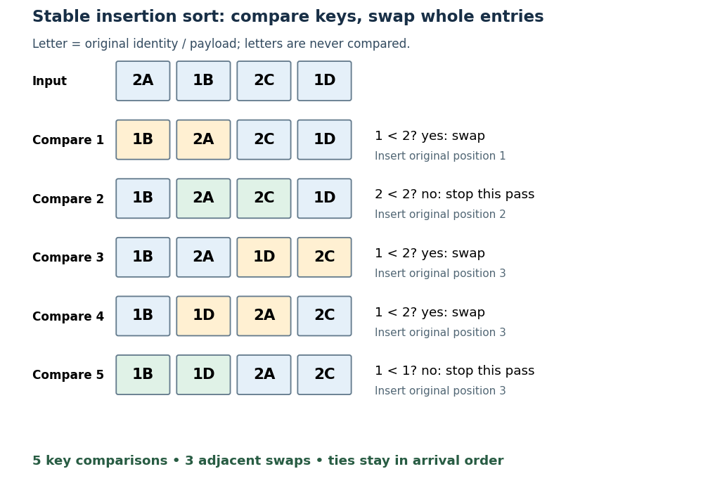
The loop invariant is that, before pass , positions satisfy sortedness and contain precisely the entries originally in that prefix. Moving the next entry left through strictly larger sort keys extends that prefix, and every swap retains sorting permutation preservation. Equal-key entries never cross, giving stable sorting. Each leftward step decreases the position, and each completed pass increases the prefix length, so the algorithm terminates.
With constant-cost key comparisons and swaps, reverse-ordered distinct sort keys cause comparisons and swaps. Thus worst-case time complexity is in Big O notation. An already sorted array needs only key comparisons for and no swaps. The adjacent-swap version uses constant auxiliary space complexity. Small or nearly sorted arrays can therefore make insertion sort useful despite its quadratic worst case.
A comparison sort learns the ordering of sort keys only by comparing pairs. The keys are otherwise opaque: their numeric values, digits or encodings cannot choose an array index or a branch. It may move complete sorting records and retain previous answers. Merge sort and the adjacent-swap insertion sort are comparison sorts; counting sort and radix sort exploit additional information.
Any deterministic comparison sort correct for all orders of distinct sort keys needs at least comparisons on some input. Here is a factorial, a logarithm, and the brackets denote the ceiling function. This is a worst-case requirement, not a requirement on every input.[ref]
For three distinct sort keys, the diagram has one leaf for each possible ordering of the original entries . Some paths need two comparisons, others three; two comparisons cannot distinguish all six orders.
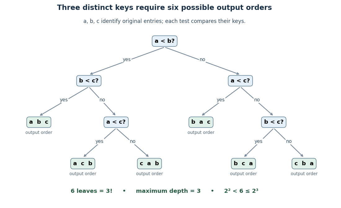
For the proof outline, represent adaptive comparisons by a binary tree: distinct sort keys give only two outcomes per comparison. A leaf fixes an output permutation; one leaf cannot correctly handle two different strict orders. Hence there must be at least leaves. Maximum depth permits at most leaves, so gives the bound. Even a three-way comparator has only two reachable outcomes on this distinct-key family.
The growth follows without a precise approximation to the factorial. At least of its factors are at least , so for ,The brackets denote the floor function. This gives a constant times lower bound for large , matching the worst-case comparison growth of merge sort.
Distinct sort keys are essential to the counting argument. Identical sort keys do not create different strict orders. If all sort keys coincide, stable sorting returns the arrival order. This does not remove the worst-case bound for a comparison sort required to handle arbitrary distinct-key inputs.
Counting sort uses integer sort keys in directly as indices into an array of counts. Constant-cost counting and indexing give time complexity in Big O notation. To retain complete sorting records, cumulative counts locate their output ranges; filling each range from its end while scanning the input backwards gives stable sorting. Emitting bare sort keys from counts would discard associated data. The term matters when the key range is large.[ref]
Radix sort sorts encoded sort keys a digit at a time. Its least-significant-digit version uses stable sorting on each successive digit, often by counting sort. For digits with possible values each, it takes time complexity in Big O notation, assuming constant-cost digit extraction and indexing. Stable sorting retains the ordering established by earlier digits when a later digit ties. Both digit access and the direct indexing in counting sort lie outside the comparison sort model, so these bounds do not contradict the comparison sorting lower bound.[ref]
Stable sorting preserves the original relative order of entries with equal keys. The entries may carry different names or other information even when their keys coincide. For example, sorting records by the numerical key gives : Ada remains before Cy. This is useful when a previous ordering contains information worth retaining, such as arrival order among equally ranked requests.
Merge sort is a divide-and-conquer algorithm that sorts a finite array by splitting it into contiguous halves, sorting each half using recursion, and combining the two sorted arrays with the merge algorithm. An empty or one-entry array is returned immediately. For length , put the first entries on the left and the remaining on the right; the brackets are the floor function and ceiling function. Always choose the left head on equal keys to obtain stable sorting. This is the split, sort, combine structure taught in the MIT lecture notes.[ref]
Take the concrete input arrayThe tags identify the entries originally at indices and , counting from zero. Both keys are ; the tags are never compared. Reading downward in the figure follows the splits, then the returned sorted arrays. Arrows show dependencies; the level layout groups independent calls rather than giving their chronological execution order.
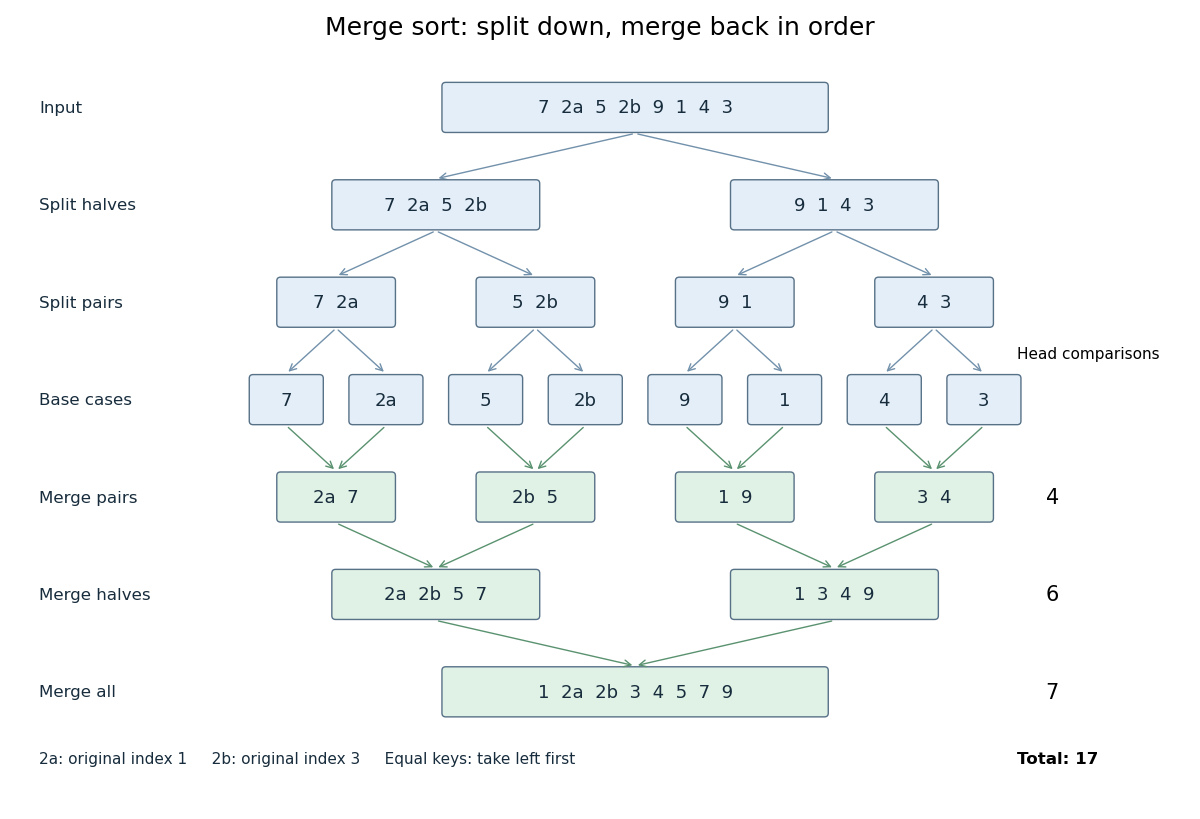
Merge sort splits into base cases and returns sorted arrays
. The tagged keys 2a and 2b retain their original order through stable sorting. The merge algorithm makes 4, 6 and 7 head comparisons on the three returning levels, for 17 in total. Details.The first two halves are and . Their pairs split into one-entry base cases. Applying the merge algorithm gives the following fully worked return levels; each number in the last column counts only comparisons between two available heads.
| Returning level | Resulting sorted arrays | Head comparisons |
|---|---|---|
| Pairs | , , , | |
| Halves | , | |
| Whole array |
In the left-half merge algorithm, the head pairs are , and ; it takes , then appends . In the final merge algorithm, the head pairs are , , , , , and . It takes , then appends . Thus this precise version makes head comparisons and, ignoring identity tags, returns .
The elegance of merge sort is that it creates exactly the structure its next step needs: two smaller sorted arrays make the larger ordering inexpensive. Once the whole array is sorted, equal keys are adjacent and binary search can serve repeated queries. Stable sorting also retains information that the keys alone do not express. If the left-half merge algorithm instead takes the right head on the tie, it returns ; the keys are sorted but stable sorting has failed.
For time complexity, assume each key comparison, entry access and entry copy has constant cost. The merge algorithm processes entries in time. In Big O notation, the resulting recurrence relation isFor , the balanced levels contain entries each and there are returning levels. Each costs , so the worst-case time complexity is . For arbitrary , there are at most returning levels, each processing at most entries, giving the same bound. The worst-case number of head comparisons is also . Here is the base-two logarithm. The MIT notes give this level-by-level analysis for merge sort.[ref]
https://ocw.mit.edu/courses/6-006-introduction-to-algorithms-spring-2020/6d1ae5278d02bbecb5c4428928b24194_MIT6_006S20_lec3.pdf. MIT 6.006 (2020), lecture 3, page 5: merge sort analysis
The conventional array implementation uses a reusable buffer of entries for the merge algorithm, together with pending calls for recursion. Its auxiliary space complexity is therefore , beyond the original array. This bound describes that implementation. A linked list permits a merge algorithm that reconnects existing nodes; its storage accounting differs from copying array entries into a buffer.
For a short algorithm correctness outline, the empty and one-entry base cases are sorted. Assuming recursion correctly sorts both shorter halves, the merge algorithm returns all their entries in order. Equal keys within a half keep their relative order by the same argument applied to the smaller call; across halves, every left entry originally preceded every right entry, so taking left first preserves stable sorting. Both half-lengths decrease for , establishing termination.
The merge algorithm combines two finite sorted sequences under the same total order, retaining every entry exactly once. Keep a position at the first unconsumed entry, or "head", of each input. While both heads exist, compare their keys, append the smaller head to the output, and advance only that head's position. On equality take the left head. Once either sequence is exhausted, append the other remainder without further key comparisons. Empty inputs therefore require no head comparisons. The MIT notes illustrate this two-head combination step.[ref]
https://ocw.mit.edu/courses/6-006-introduction-to-algorithms-fall-2011/90a37c49b07b105ea7a027abc67eddc6_MIT6_006F11_lec03.pdf. MIT 6.006 (2011), lecture 3: merging sorted arrays
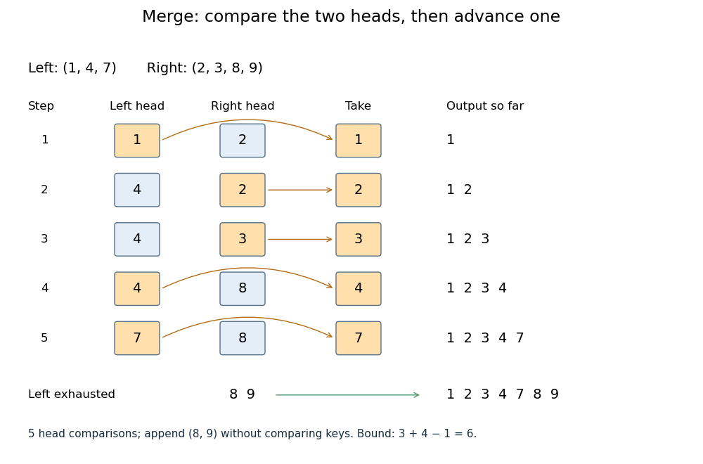
Five head comparisons in the merge algorithm
. Orange heads are chosen and arrows lead to the next output entry. The compared head pairs are (1,2), (4,2), (4,3), (4,8) and (7,8). The left sequence then runs out; append (8,9) without further key comparisons. Details.The head pairs , , , and select respectively. After the fifth comparison the left sequence is empty, so is appended. Seven entries are written, but only five head comparisons occur: tests for exhaustion and appending the remainder are separate operations. This distinction makes the example's count smaller than the bound .
For nonempty inputs of lengths , each head comparison consumes exactly one entry. After such removals at most one entry remains, so both heads cannot still exist. Hence the merge algorithm uses at most head comparisons. The bound can be attained: and require six head comparisons before the left sequence is exhausted. With constant-cost comparisons, access and copying, writing all entries gives time complexity in Big O notation. Writing a separate output array needs entry slots; the two positions require only constant additional storage.
The merge algorithm is useful whenever two already ordered collections must become one: it reads each input only forwards. This works with arrays and linked lists, without needing access to arbitrary middle positions. Choosing left on ties preserves each input's internal order and places equal left entries before equal right entries, which is the combination rule needed for stable sorting in merge sort.
The loop invariant behind algorithm correctness is that the emitted prefix is sorted, contains exactly the consumed entries, and every emitted key is at most every unconsumed key. Each sorted sequence has its smallest remaining key at its head, so the smaller of the two heads is safe to append. The invariant survives each removal; when one sequence ends, the other sorted remainder is safe to append in full. Each comparison removes an entry, so termination follows from the finite input lengths.
// Target: computer-science.bigb
Binary search finds a target in a sorted array by inspecting the middle of the remaining candidate range. If the middle entry is smaller than , every entry to its left is also too small; if larger, every entry to its right is too large. One comparison therefore rules out many entries. Equal entries are allowed; this version returns any matching index, without promising the first occurrence.
Use indices starting at zero and inclusive endpoints . Initially , , where is the array length. While , chooseThe brackets denote the floor function. Compare with : return on equality; set if ; otherwise set . If , report absence. The updates exclude the already inspected middle entry. This also handles an empty array, whose initial endpoints are . Sedgewick and Wayne specify a sorted array as input and return a matching index or for absence.[ref]
https://algs4.cs.princeton.edu/code/javadoc/edu/princeton/cs/algs4/BinarySearch.html. Sedgewick and Wayne: BinarySearch API
For , the first two steps agree. Next retains only index ; inspecting sets . Now , so the answer is "absent" after four comparisons.
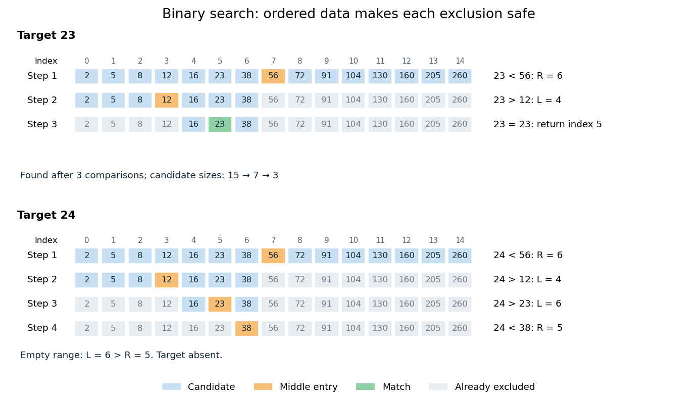
Binary search retains only candidates compatible with every comparison
. Blue cells are current candidates, orange marks the middle entry, and green marks a match. Both searches use the same fifteen-entry sorted array. Details.The loop invariant is: the array stays sorted, , and every index containing lies between and . It holds initially. The sorted array property justifies each exclusion. Returning on equality gives a match; an empty candidate range implies absence. Crucially, this loop invariant allows to be absent from the beginning.
For a nonempty range of size , an unsuccessful comparison leaves at most candidates. Thus sizes satisfy after unsuccessful comparisons. This proves termination and, for , at most middle-entry comparisons. The final singleton still needs inspection: requires one comparison, not zero. For , the bound is four. This is the halving argument behind logarithmic time complexity.[ref]
https://www.cs.princeton.edu/courses/archive/fall24/cos126/static/lectures/42Algorithms.pdf. Princeton COS 126: binary search analysis
A decision tree with binary tests has at most leaves. Distinguishing possible matching positions therefore requires . This lower bound counts binary tests, whereas the bound above counts three-way comparisons.
Karatsuba multiplication is a divide-and-conquer algorithm for multiplication of integers. Splitting each operand into two blocks seems to require four smaller products; the Karatsuba three-product identity recovers the two cross terms together from just three products. Repeating that saving through recursion changes the time complexity from quadratic to , where counts digits in a fixed positional notation. The exponent is about : the benefit comes from the algorithm, even though each splitting step needs more addition and subtraction.
The Karatsuba worked multiplication below computes using , , and . The last operand already shows why “half-size” needs care: Karatsuba carry handling and Karatsuba recursion termination account for the extra digit. Karatsuba digit-operation cost states the operation model; Karatsuba practical crossover explains why the asymptotic saving alone does not select a useful threshold.
The original 1962 paper presents a binary numeral system automaton construction: its Theorem 2 and proof reduce multiplication to taking squares of numbers, then reduce a larger square of a number to three smaller squares of numbers. Its footnote explicitly addresses the extra digit in a sum of halves. The sequential time complexity analysis below uses a different operation model from that paper's automaton size and depth bounds, including its Boolean circuit realization without feedback.[ref]
Multiplication of many-digital numbers by automatic computers by A. Karatsuba and Yu. Ofman. Karatsuba and Ofman, Multiplication of many-digital numbers by automatic computers, original Russian article, 1962, pp. 293–294: Theorem 2, its proof, and the footnote on p. 294
Fix an integer base . Let have at most digits in positional notation, treating zero as one digit. For , set using the ceiling function, and . Euclidean division giveswhere and . The floor function selects the high block; the remainder selects the low block. Both operands must use the same , including when their actual digit lengths differ.
For odd , the low block has digit positions and the high block has . Leading zero padding aligns a shorter operand without changing its integer value. Padding to a power-of-two length is optional: the split itself works for every . If power-of-two padding is used, the padded length is less than twice the original length, so it changes only a constant factor in the asymptotic analysis.
Compute exactly three smaller products,The distributive property gives , so the cross coefficient is . Recombine byThe saving is that and are never separately multiplied. Multiplying a digit block by or shifts its position in positional notation; it does not require another general integer multiplication. Addition of the shifted results still requires Karatsuba carry handling.
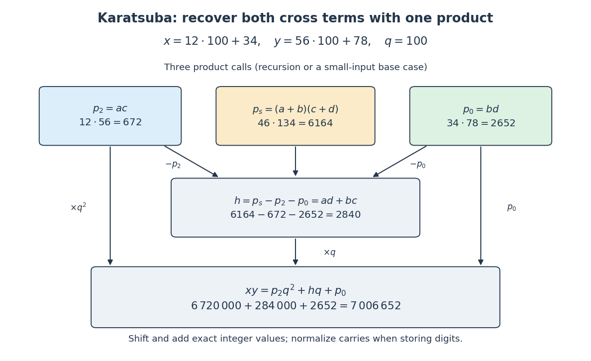
Three products recover the Karatsuba cross coefficient
. The arrows carry exact integer values for the Karatsuba worked multiplication. Only the three coloured product boxes require recursive multiplication; the lower boxes use subtraction, digit shifts and addition. Details.Use decimal expansion, , , , and . The Karatsuba operand splitting is , . The Karatsuba three-product identity givesThe third product has a three-digit operand. A small-input base case can evaluate these three products directly, or a smaller threshold can continue recursion. Either choice preserves the identity; only the operation count changes.
The same Karatsuba operand splitting handles : choose , , and write , . Then , , , and , giving . A zero high block and unequal lengths require no new algebraic rule.
The blocks in the Karatsuba three-product identity are integers, not single digits: can need positions and can exceed . Concatenating the displayed blocks therefore fails. Accumulate their shifted values with ordinary addition, normalizing each digit position by Euclidean division: a coefficient becomes the digit , with carry passed to the next position. Subtraction likewise propagates borrows. Although for these nonnegative integers, intermediate digitwise subtraction can still borrow.
In the four-digit Karatsuba worked multiplication, grouping by base gives unnormalized coefficients , written from high to low. Normalize from the right: ; ; . The final groups are , yielding . The zero group must retain its two positions.
Since , their sums are less than and can need digits. Allocate that extra digit before the third recursive product; discarding it can change the answer. The GMP manual describes this sum growth and uses a difference-based form to avoid it.[ref]
Karatsuba Multiplication. GNU MP 6.3.0 manual, §15.1.2 Karatsuba Multiplication: sum-based middle product can exceed k limbs; absolute differences and their signs
For the sum-based Karatsuba three-product identity, a safe fixed base-case threshold is three digits or more. Return zero directly if either operand is zero; at or below the threshold, use ordinary digit-by-digit multiplication. Otherwise split by the maximum current operand length and invoke Karatsuba multiplication on , , and .
Each recursive operand has at most digits. This is strictly less than for , proving termination. A rule stopping only at one digit does not supply this guarantee: in base two, splits into , whose sum is , still two digits. An implementation must choose a sufficient threshold or explicitly handle such nonshrinking calls. Leading zero padding must not be repeatedly added in a way that defeats the decreasing size measure.
For signed integers, multiply absolute values with the same nonnegative procedure and restore the sign afterwards. This changes the representation bookkeeping, rather than the three-product identity.
Count a fixed-base digit addition, subtraction, digit copy, or single-digit multiplication as constant cost. Base stays fixed as grows; an entire arbitrary-length integer multiplication is not one constant-cost step. With this model, splitting, sum formation, shifts and recombination require digit operations. Ordinary digit-by-digit multiplication forms digit products for two -position operands. The GMP base-case description uses this rectangular product arrangement.[ref]
Basecase Multiplication. GNU MP 6.3.0 manual, §15.1.1 Basecase Multiplication: rectangular cross-products and O(NM) cost
The ideal equal-half recurrence relation isFor , level has calls of size . If each internal call incurs exactly times its size in additional digit work, that level contributes . There are leaves. The geometric series of internal work isThus fixed positive leaf cost plus this internal work grows on the order of . In Big O notation, . Removing one of four products at every level matters much more than saving just one at the root.
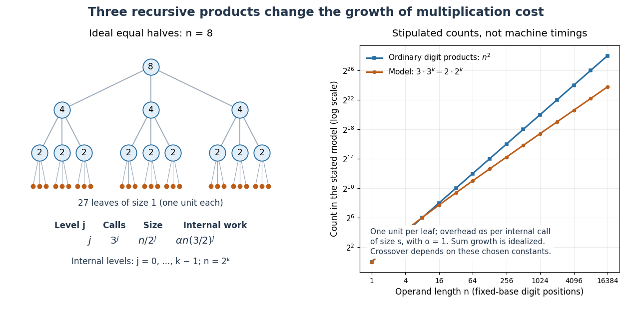
Karatsuba recursion levels and an explicitly stipulated cost comparison
. Left: the ideal equal-half recursion for , with three children per internal call. Right: model counts for , one unit per leaf and internal overhead for size with . The resulting count is , compared with ordinary digit products. This illustrates the recurrence relation; its constants and crossover are stipulated, rather than measured execution times. Details.The literal sum-based implementation instead admits the upper boundfor a nondecreasing worst-case cost envelope above a fixed base-case threshold. The extra digit does not change the exponent: since , subtracting three from the size makes each child's adjusted size at most half its parent's. Stop this comparison at any fixed threshold greater than three; its recursion depth is and the level-work sum is bounded by the same geometric series up to constant factors. Exact call counts can depend on carries, zero shortcuts and the threshold, so they need not equal the ideal at each depth.
Karatsuba digit-operation cost explains eventual scaling, while a practical base-case threshold depends on the costs of addition, subtraction, copying and function calls relative to small integer multiplication. Using for a base-case cost, one Karatsuba level costs : the quadratic coefficient falls to , but the linear contribution includes . Small operands can therefore cost more despite the smaller exponent. This comparison and the effect of implementation improvements on the threshold are described in the GMP manual.[ref]
The plotted crossover belongs only to the stipulated constants in its caption; its ordinary-method curve counts digit products alone, while the Karatsuba curve includes the chosen internal overhead. Selecting a threshold for real software requires measuring the actual implementation on its intended machine. With base for a fixed machine digit width , the same analysis counts machine digits; it does not establish a universal crossover in decimal digits, bits, or elapsed time.
Derandomization converts a randomized construction or algorithm into a deterministic one while preserving its desired guarantee. The method of conditional probabilities does this by maintaining a computable conditional expectation until all choices are fixed.
For a random objective with an easily computable conditional expectation, reveal one random choice at a time and choose an outcome whose conditional expected objective is at least the current value. Such an outcome exists because the current value is an average of the child values. When all choices are fixed, the actual objective is at least the initial expectation. Biased as well as fair choices work. Efficient expectation updates make the resulting deterministic procedure a polynomial-time algorithm.
A probabilistic Turing machine is a Turing machine whose transitions may depend on independent random bits.
A randomized decision algorithm has one-sided error when one answer is always correct and only the other answer can be mistaken.
contains decision problems with a polynomial-time randomized algorithm that rejects every negative instance and accepts every positive instance with probability at least one half.
consists of complements of languages in RP. Its algorithms always accept positive instances and reject negative instances with probability at least one half.
. Equivalently, it consists of problems having an always-correct randomized algorithm with polynomial expected running time.
Independent repetitions reduce a randomized algorithm's error probability while preserving polynomial running time.
Polynomial identity testing asks whether a polynomial represented implicitly, such as by an arithmetic circuit or a remainder computation, is the zero polynomial.
Articles by others on the same topic

An algorithm is a finite sequence of well-defined instructions or steps designed to perform a specific task or solve a particular problem. Algorithms can be expressed in various forms, including natural language, pseudocode, flowcharts, or programming code. Key characteristics of algorithms include: 1. **Clear and Unambiguous**: Each step must be precisely defined so that there is no uncertainty about what is to be done.



