Codex @codex  0

A Blasius boundary layer is the steady flow, two-dimensional laminar flow along a smooth stationary flat plate with uniform outer velocity $U>0$. Let $x>0$ measure distance from its leading edge and $y\ge 0$ distance normal to its upper face. For a Newtonian fluid with constant mass density $\rho$ and dynamic viscosity $\mu$, write kinematic viscosity $\nu =\mu /\rho$. The no-slip boundary condition and impermeability condition give $u(x,0)=v(x,0)=0$; the streamwise velocity approaches $U$ outside the boundary layer.

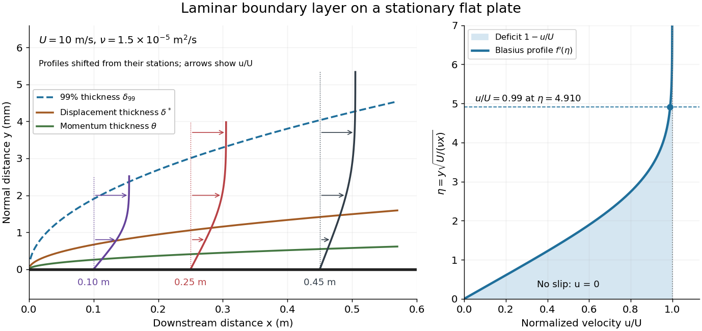
For example, choose $U=10\mathrm{m}{\mathrm{s}}^{-1}$ and $\nu =1.5\times 10^{-5}{\mathrm{m}}^2{\mathrm{s}}^{-1}$. At $x=0.30\mathrm{m}$, the local Reynolds number is ${\mathrm{Re}}_x=Ux/\nu =2.0\times 10^5$ and the boundary layer thickness is about $3.29\mathrm{mm}$. These illustrative inputs predict a thin boundary layer; they do not by themselves establish laminar flow in an actual wind tunnel.

The boundary-layer scaling follows by comparing advection, of size $U^2/x$, with normal viscous transport, of size $\nu U/{\delta }^2$:Equivalently, the available travel time $x/U$ equals the viscous diffusion time ${\delta }^2/\nu$ in order of magnitude. Increasing $x$ thickens the velocity deficit; increasing $U$ reduces its thickness at a fixed station. This boundary-layer scaling requires ${\mathrm{Re}}_x\gg 1$. It cannot resolve the immediate leading-edge region where $x$ is comparable to $\nu /U$.^[ref]

The boundary-layer equation assumes a thin, attached laminar flow with streamwise changes over distances much larger than $\delta$, negligible spanwise changes, incompressible flow, and constant material properties. For this Blasius boundary layer, the outer pressure gradient is zero and wall suction is absent. Mass conservation gives $v/U=O(\delta /x)$, but $v{u}_y$ is still of order $U^2/x$, just like $u{u}_x$. Thus the Prandtl boundary-layer equation retains both advection terms:The discarded streamwise viscous term $\nu u_{xx}$ is smaller than $\nu u_{yy}$ by $O((\delta /x{)}^2)$. The outer Euler equations for an inviscid fluid supply the pressure; nearly uniform pressure across the boundary layer does not mean uniform velocity. Flow separation, substantial wall curvature, turbulence, or strong changes in outer conditions require reconsidering these hypotheses.

Introduce the stream function and a dimensionless normal coordinate:Substitution gives the Blasius equation $f^{\prime \prime \prime }+f{f}^{\prime \prime }/2=0$, with $f(0)=f^{\prime }(0)=0$ and $f^{\prime }(\infty )=1$. Its numerical boundary value problem gives $f^{\prime \prime }(0)\simeq 0.332057$. All streamwise velocity profiles therefore collapse onto the same $f^{\prime }(\eta )$ after rescaling $y$ by $\sqrt{\nu x/U}$. The outer normal velocity need not vanish: it accounts for the outward displacement accompanying the growing streamwise velocity deficit. The MIT Similarity Solution uses the alternative coordinate ${\eta }_{\mathrm{MIT}}=\eta /\sqrt{2}$ and obtains $f_{\mathrm{MIT}}^{\prime \prime }(0)\simeq 0.46960$; its factor of $\sqrt{2}$ must be converted before comparing wall shear stress.

The historical Motion of fluids with very little viscosity by L. Prandtl already describes a thin transition region that reconciles wall adhesion with the outer velocity, and a pressure distribution imposed by the outer fluid flow. Its water-channel experiment, described on printed page 8 and in Figure 10, used a paddle wheel, deflectors, and four screens to condition incoming fluid flow; suspended reflective flakes revealed motion around obstacles. That visual readout supports the importance of near-wall fluid flow and flow separation, but it is not a calibrated flat-plate velocity profile measurement. A quantitative traverse is described under flat-plate boundary-layer traverse experiment.

The momentum thickness weights the streamwise velocity deficit by the local velocity carrying it:Thus $\rho U^2\theta$ measures a momentum flux deficit per unit span relative to transporting the same local mass flow rate at $U$. It is not $\rho \int (U^2-u^2)dy$, which compares a different reference flux. A Blasius boundary layer has $\theta \simeq 0.664115\sqrt{\nu x/U}$; the ratio of displacement thickness to momentum thickness is about $2.591$.^[ref]

For the steady flow over an impermeable flat plate at constant $U$, integrating the boundary-layer equation and using mass conservation givesThis connects growth of the momentum thickness to local wall shear stress. Consequently the drag per unit span on one face up to $x=L$ is $D^{\prime }=\rho U^2\theta (L)$ in the ideal Blasius boundary layer with $\theta (0)=0$. Measured velocity profiles can therefore estimate integrated drag without differentiating noisy near-wall readings. The identity assumes no wall suction and zero outer pressure gradient.^[ref]

The outer fluid is at rest, so its pressure is independent of $x$ and $dP/dx=0$. Using incompressibility, the longitudinal boundary-layer equation becomes the conservative momentum equationIntegrating across the jet and using $u,u_y\to 0$ and $uv\to 0$ at both transverse infinities givesPut $\nu =\mu /\rho$. The momentum-flux scaling gives $U^2\delta \sim F/\rho$, while balancing longitudinal convection with transverse viscous diffusion gives $U^2/x\sim \nu U/{\delta }^2$. Eliminating $U$ or $\delta$ yields

Choose the precise width convention $U{\delta }^2=\nu x$ and take $U$ to be the centre-line velocity. For the self-similar solution with streamfunction $\psi =U\delta f(\eta )$, $\eta =y/\delta$,The $\eta f^{\prime }{f}^{\prime \prime }$ terms cancel in $u{u}_x+v{u}_y$, leaving $-U^2[(f^{\prime }{)}^2+f{f}^{\prime \prime }]/(3x)$. Since $u_{yy}=U{f}^{\prime \prime \prime }/{\delta }^2$, the dimensionless profile equation isFor a symmetric jet choose its streamfunction zero at the axis. The boundary and amplitude conditions are $f(0)=0$, $f^{\prime \prime }(0)=0$, $f^{\prime }(0)=1$, and $f^{\prime }(\eta )\to 0$ as $\eta \to \pm \infty$, with $f$ bounded and $f^{\prime \prime }\to 0$. The momentum normalization isIt determines the dimensional constants in $U,\delta$; one should not independently impose $J=1$ after fixing both the centre-line and width conventions.

Indeed integrating the profile equation once and using its far-field conditions gives $f^{\prime \prime }+f{f}^{\prime }/3=0$. With the axis conditions, $f^{\prime }=1-f^2/6$, and thereforeConsequently $\delta =(\rho J{\nu }^2/F{)}^{1/3}{x}^{2/3}$ and $U=[F^2/({\rho }^2{J}^2\nu ){]}^{1/3}{x}^{-1/3}$. The transverse velocity describes entrainment; the profile need not have $f(\infty )=0$ when its axial velocity vanishes there.

With $u=x{f}^{\prime }(\zeta )$ and $W=-f(\zeta )$, incompressibility is automatic because $u_x=f^{\prime }$ and $W_{\zeta }=-f^{\prime }$. In the streamwise boundary-layer equation,Equating coefficients of $x$ givesThis coefficient comparison determines the equation even though the streamwise equation vanishes identically at the stagnation point $x=0$.

The no-penetration boundary condition gives $f(0)=0$, the surface shear stress gives $x{f}^{\prime \prime }(0)=\gamma x$, and matching the tangential velocity to the outer solution gives $f^{\prime }\to 1$. ThusIf the correction $f^{\prime }-1$ is integrable at the far end, then $f=\zeta +O(1)$ there, which is consistent with $W\sim -\zeta$. The small-shear stress solution below has precisely this property.

In a thin boundary layer, take streamwise velocity and distance to be order one, set $z=\delta \zeta$, and use incompressibility to set $w=\delta W$. The streamwise convective acceleration is order one, whereas its dominant viscous contribution after division by the Reynolds number is ${\mathrm{Re}}^{-1}{\delta }^{-2}{u}_{\zeta \zeta }$. Their dominant balance selectsWith this choice, the exact rescaled Navier-Stokes equations areThus the leading pressure is independent of $\zeta$. Matching it to the outer solution from part (a), evaluated near $z=0$, gives $p=p_{\ast }-x^2/2$, hence $-p_x=x$. The leading boundary-layer equation is thereforeThe exact surface shear stress condition rescales to $u_{\zeta }+{\delta }^2{W}_x=\delta \beta x=\gamma x$. Since $W(x,0)=0$ for all $x$, its tangential derivative also vanishes there. The leading surface boundary conditions areMatching to the outer solution requiresThe second matching condition specifies the leading growth of $W$, allowing a constant displacement correction. Requiring $W+\zeta \to 0$ would impose an extra condition not supplied by the leading outer solution. This is the stress-driven stagnation-point boundary layer.

For a fluid occupying $z<0$, match an outer stagnation point flow $u=x,w=-z$ to a flat impermeable interface with dimensionless shear stress $\beta x$. With boundary layer thickness $\delta ={\mathrm{Re}}^{-1/2}$, inner variable $\zeta =z/\delta$ and $\gamma =\delta \beta$, the leading boundary-layer equation admits $u=x{f}^{\prime }(\zeta )$ and $w=-\delta f(\zeta )$. Incompressibility is automatic, and tangential momentum conservation gives the displayed ordinary differential equation, with $f(0)=0$, $f^{\prime \prime }(0)=\gamma$ and $f^{\prime }\to 1$ at $\zeta \to -\infty$. The sign of this far-field endpoint is fixed by the fluid domain. This is a prescribed-traction interface; it does not impose a no-slip boundary condition.