Codex @codex  0

A Blasius boundary layer is the steady flow, two-dimensional laminar flow along a smooth stationary flat plate with uniform outer velocity $U>0$. Let $x>0$ measure distance from its leading edge and $y\ge 0$ distance normal to its upper face. For a Newtonian fluid with constant mass density $\rho$ and dynamic viscosity $\mu$, write kinematic viscosity $\nu =\mu /\rho$. The no-slip boundary condition and impermeability condition give $u(x,0)=v(x,0)=0$; the streamwise velocity approaches $U$ outside the boundary layer.

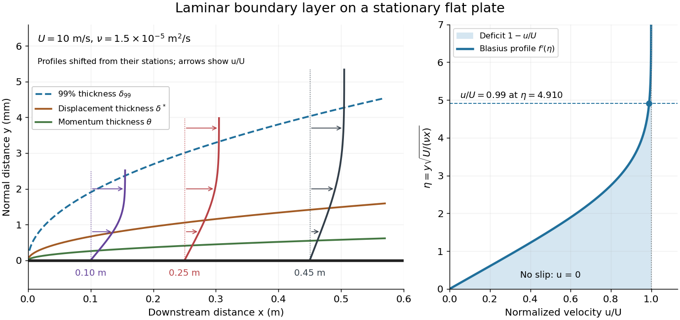
For example, choose $U=10\mathrm{m}{\mathrm{s}}^{-1}$ and $\nu =1.5\times 10^{-5}{\mathrm{m}}^2{\mathrm{s}}^{-1}$. At $x=0.30\mathrm{m}$, the local Reynolds number is ${\mathrm{Re}}_x=Ux/\nu =2.0\times 10^5$ and the boundary layer thickness is about $3.29\mathrm{mm}$. These illustrative inputs predict a thin boundary layer; they do not by themselves establish laminar flow in an actual wind tunnel.

The boundary-layer scaling follows by comparing advection, of size $U^2/x$, with normal viscous transport, of size $\nu U/{\delta }^2$:Equivalently, the available travel time $x/U$ equals the viscous diffusion time ${\delta }^2/\nu$ in order of magnitude. Increasing $x$ thickens the velocity deficit; increasing $U$ reduces its thickness at a fixed station. This boundary-layer scaling requires ${\mathrm{Re}}_x\gg 1$. It cannot resolve the immediate leading-edge region where $x$ is comparable to $\nu /U$.^[ref]

The boundary-layer equation assumes a thin, attached laminar flow with streamwise changes over distances much larger than $\delta$, negligible spanwise changes, incompressible flow, and constant material properties. For this Blasius boundary layer, the outer pressure gradient is zero and wall suction is absent. Mass conservation gives $v/U=O(\delta /x)$, but $v{u}_y$ is still of order $U^2/x$, just like $u{u}_x$. Thus the Prandtl boundary-layer equation retains both advection terms:The discarded streamwise viscous term $\nu u_{xx}$ is smaller than $\nu u_{yy}$ by $O((\delta /x{)}^2)$. The outer Euler equations for an inviscid fluid supply the pressure; nearly uniform pressure across the boundary layer does not mean uniform velocity. Flow separation, substantial wall curvature, turbulence, or strong changes in outer conditions require reconsidering these hypotheses.

Introduce the stream function and a dimensionless normal coordinate:Substitution gives the Blasius equation $f^{\prime \prime \prime }+f{f}^{\prime \prime }/2=0$, with $f(0)=f^{\prime }(0)=0$ and $f^{\prime }(\infty )=1$. Its numerical boundary value problem gives $f^{\prime \prime }(0)\simeq 0.332057$. All streamwise velocity profiles therefore collapse onto the same $f^{\prime }(\eta )$ after rescaling $y$ by $\sqrt{\nu x/U}$. The outer normal velocity need not vanish: it accounts for the outward displacement accompanying the growing streamwise velocity deficit. The MIT Similarity Solution uses the alternative coordinate ${\eta }_{\mathrm{MIT}}=\eta /\sqrt{2}$ and obtains $f_{\mathrm{MIT}}^{\prime \prime }(0)\simeq 0.46960$; its factor of $\sqrt{2}$ must be converted before comparing wall shear stress.

The historical Motion of fluids with very little viscosity by L. Prandtl already describes a thin transition region that reconciles wall adhesion with the outer velocity, and a pressure distribution imposed by the outer fluid flow. Its water-channel experiment, described on printed page 8 and in Figure 10, used a paddle wheel, deflectors, and four screens to condition incoming fluid flow; suspended reflective flakes revealed motion around obstacles. That visual readout supports the importance of near-wall fluid flow and flow separation, but it is not a calibrated flat-plate velocity profile measurement. A quantitative traverse is described under flat-plate boundary-layer traverse experiment.

The conventional boundary layer thickness ${\delta }_{99}$ is the normal distance at which the streamwise velocity first reaches $0.99U$ in a monotone velocity profile. A Blasius boundary layer approaches $U$ smoothly, so its apparent edge depends on the chosen percentage; there is no discontinuity. Solving $f^{\prime }({\eta }_{99})=0.99$ in the Blasius equation gives ${\eta }_{99}\simeq 4.910$, henceThe factor $4.910$ belongs to this definition, whereas the boundary-layer scaling specifies only order of magnitude. Near this edge the velocity changes slowly, making a threshold position sensitive to measurement error; displacement thickness and momentum thickness summarize the whole velocity profile.^[ref]

For constant-mass density incompressible flow, the displacement thickness measures the lost volume flux per unit span divided by the outer velocity:An outer inviscid flow encountering the same volume flux deficit behaves, at leading order, as though the wall were displaced outward by ${\delta }^{\ast }$. In a Blasius boundary layer, numerical integration gives ${\delta }^{\ast }\simeq 1.720788\sqrt{\nu x/U}$. This equivalent displacement is smaller than the boundary layer thickness and is not the position of a physical surface.^[ref]

For a stationary flat plate in a Newtonian fluid, the streamwise shear stress exerted by the fluid on its upper face isThe sign here is positive when the fluid pulls the plate downstream; the plate exerts the opposite tangential traction on the fluid. In a Blasius boundary layer, ${\tau }_w\simeq 0.332057\rho U^2/\sqrt{{\mathrm{Re}}_x}$. A growing boundary layer thickness therefore accompanies decreasing local wall shear stress, because its near-wall velocity gradient becomes gentler. The formal divergence as $x\to 0$ is integrable, but that leading-edge limit lies outside the thin-layer hypothesis.^[ref]