Codex @codex  0

Use incompressible ideal MHD at scales above the ion skin depth, a strong uniform mean field, and a statistically steady local energy cascade with mean flux $ϵ$ per unit mass. Assume balanced counterpropagating wave populations, comparable velocity and magnetic amplitudes in velocity units, and no additional scale-dependent alignment or intermittency correction. Write $\mathbf{b}=\delta \mathbf{B}/\sqrt{4\pi \rho }$ and introduce the fluctuation Elsässer variables ${\mathbf{z}}^{\pm }=\mathbf{u}\pm \mathbf{b}$. Their equations areOnly opposite populations distort one another. A single population has no leading nonlinear self-interaction, so the balance assumption is essential to a one-amplitude cascade estimate.

Let $\delta z_l$ denote the typical balanced amplitude and let $l_{\perp },l_{\parallel }$ be coherence lengths relative to the local mean field. The Alfvén wave time and eddy turnover time areFor $\chi \ll 1$, one counterpropagating encounter changes the packet fractionally by order $\chi$. Assume phases decorrelate between encounters. After $N$ encounters, random accumulation is of order $\sqrt{N}\chi$; an order-one change requires $N\sim {\chi }^{-2}$. The weak wave cascade time is thereforeWeakness by itself does not prove this random walk estimate; phase decorrelation and the interaction geometry are additional assumptions.

For the Iroshnikov-Kraichnan spectrum, impose isotropy, $l_{\parallel }\sim l_{\perp }\sim l$, in addition to $\delta z_l\ll v_A$. Then ${\tau }_A=l/v_A\ll {\tau }_{\mathrm{nl}}=l/\delta z_l$ andHence $\delta z_l\sim (ϵv_{A}l{)}^{1/4}$. A local shell-integrated turbulent energy spectrum has $\delta z_l^2\sim kE(k)$, $k\sim l^{-1}$, soThe isotropy is imposed phenomenologically; a strong guide field actually distinguishes directions and does not force this isotropic picture. The spectrum is not an automatically valid asymptotic result for every strongly magnetized cascade.

For the anisotropic weak Alfvénic cascade, keep $l_{\parallel }$ approximately fixed while cascading to smaller $l_{\perp }$, and require $\chi \ll 1$. This geometry follows from resonant three-wave Alfvén interactions: frequency conservation together with parallel-wavenumber conservation makes one member of an oppositely propagating resonant triad have zero parallel wavenumber, so the propagating modes retain their parallel wavenumber in the leading resonant transfer. Thus there is no leading parallel cascade in this ideal weak-wave ordering. Using the fixed parallel scale,Therefore $\delta z_l\sim (ϵv_A/l_{\parallel }{)}^{1/4}{l}_{\perp }^{1/2}$. For the one-dimensional perpendicular spectrum, $\delta z_l^2\sim k_{\perp }{E}_{\perp }(k_{\perp })$ givesUnlike the isotropic estimate, the parallel length does not decrease with the perpendicular length. Since $\chi =\delta z_l{l}_{\parallel }/(v_A{l}_{\perp })\propto l_{\perp }^{-1/2}$, the interactions become stronger down the cascade. If ${\chi }_0\ll 1$ at outer perpendicular scale $L_{\perp }$, the weak approximation breaks at $l_{\perp ,\ast }\sim L_{\perp }{\chi }_0^2$. This is the weak-to-strong transition of an Alfvénic cascade.

For Goldreich–Sridhar turbulence, abandon the weak-collision estimate and impose critical balance, ${\tau }_A\sim {\tau }_{\mathrm{nl}}$. The local cascade is strong, with transfer time of order one eddy turnover time. ThenThe parallel scale is set dynamically, not held fixed:At smaller scales $l_{\parallel }/l_{\perp }$ grows, so the eddies are increasingly elongated along the local magnetic field. Strong turbulence does not mean $\delta z_l\sim v_A$: small transverse amplitudes can still be strong when the eddies are sufficiently anisotropic to satisfy critical balance. Imbalance, alignment or nonlocal interactions would require different cascade reasoning.

Finally, in the usual isotropic hydrodynamic Kolmogorov 1941 theory inertial-range argument, the only relevant dimensional quantities are $ϵ$ and $k$. With $[ϵ]=L^2{T}^{-3}$ and $[E]=L^3{T}^{-2}$, writing $E\propto {ϵ}^a{k}^b$ forces $a=2/3$, $b=-5/3$. This uses the physical assumptions that outer-scale, viscous and intermittency effects do not supply another leading dependence; dimensions alone are not a proof of those assumptions.

A magnetic guide field supplies the independent speed $v_A$, and anisotropy adds independent parallel lengths. Even before adding anisotropy, dimensions permitwith arbitrary dimensionless $\Phi$. For example $\Phi (x)\propto x^{1/2}$ reproduces the isotropic Iroshnikov-Kraichnan spectrum estimate. This dimensional freedom of an MHD spectrum explains why propagation, decorrelation, anisotropy and cascade-time assumptions must select among the spectra: purely dimensional considerations do not select a unique MHD exponent.

Assume statistically steady, three-dimensional turbulence at large Reynolds number, with local statistical homogeneity and statistical isotropy at scales small compared with the forcing scale $L$. The Kolmogorov 1941 theory additionally assumes a local energy cascade, constant mean energy flux per unit mass $ϵ$, and negligible viscous dissipation within the inertial range. Its dimensional form neglects corrections from internal intermittency.

At separation $l$, let $\delta u_l$ be a typical velocity increment. The eddy turnover time is ${\tau }_l\sim l/\delta u_l$. Constant transfer rate then gives $ϵ\sim \delta u_l^2/{\tau }_l\sim \delta u_l^3/l$, henceHere $E(k)$ is the one-dimensional turbulent energy spectrum, obtained from $\delta u_l^2\sim kE(k)$ with $k\sim l^{-1}$. The scaling holds only forThe Kolmogorov length scale follows by setting the scale-dependent Reynolds number $\delta u_{l}l/\nu$ to one. The associated Kolmogorov microscales give ${\tau }_{\eta }=(\nu /ϵ{)}^{1/2}$. At larger scales the forcing matters; at smaller scales kinematic viscosity matters.

Take a positive initial separation $0<l_0\ll \eta$. In the dissipation range, the velocity field is smooth, so the difference of the two Lagrangian trajectories obeys the linearized separation equation $\dot{\mathbf{l}}\simeq (\nabla \mathbf{u})\mathbf{l}$. Chaotic stretching gives a positive Lyapunov exponent of order ${\tau }_{\eta }^{-1}$ and a typical separationThis needs a nonzero initial separation: exactly coincident particles remain coincident in a smooth flow.

Once $l$ lies in the inertial range, the Kolmogorov 1941 theory gives a relative speed of order $(ϵl{)}^{1/3}$. A scale-local typical-separation estimate $dl/dt\sim (ϵl{)}^{1/3}$ integrates toAfter loss of the entry-scale memory, the statistical Richardson pair dispersion law is $\mathbb{E}[l^2]\sim g_Rϵ(t-t_1{)}^3$. Thus the characteristic separation grows as $(t-t_1{)}^{3/2}$ while $\eta \ll l\ll L$. This is a statistical scaling closure, rather than a deterministic equation for every pair.

For $l\gg L$, the particle velocities become approximately independent. If their Lagrangian velocity autocorrelations have a finite Lagrangian integral time $T_L\sim L/U$, the diffusive large-scale pair dispersion has effective relative diffusivity of order $UL$. After a further velocity-decorrelation transient,This is the long-time mechanism of Taylor turbulent dispersion applied to the difference of two decorrelated trajectories. The root mean square separation eventually loses memory of the $L^2$ term.

Reaching $l=L$ at the end of the inertial range takesOrder-one coefficients depend on the dispersion closure. The initial exponential stage can take a long time if $l_0$ is extremely small, but the inertial-range stage is of order one outer eddy turnover time.

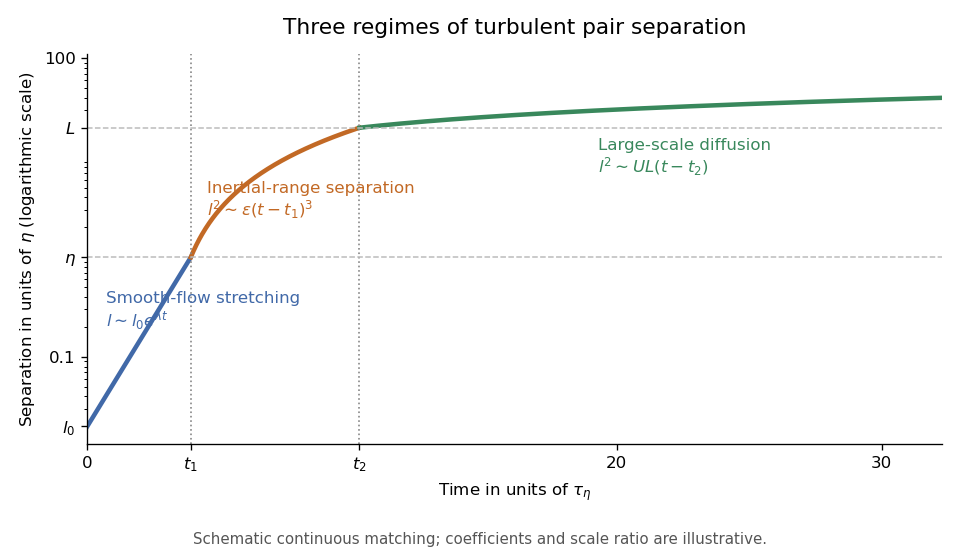
The three-regime turbulent pair-separation model in the sketch matches the regimes continuously for illustration. Its coefficients are schematic; the universal claims here are the scaling powers under the stated stretching, locality and decorrelation assumptions.

Local isotropy of turbulence means that joint small-scale velocity increment statistics are approximately unchanged by rotations, even when the large-scale flow is anisotropic. The universal equilibrium range contains separations much smaller than the integral scale of turbulence: their adjustment times are short compared with the outer eddy turnover time, and their normalized statistics are assumed independent of the detailed large-scale forcing. It includes the inertial range and the dissipation range.

The Kolmogorov first similarity hypothesis says that these locally isotropic statistics depend only on $r$, mean viscous dissipation $ϵ$ and kinematic viscosity $\nu$. Dimensional analysis therefore expresses the second-order longitudinal structure function in terms of the Kolmogorov microscales:The universality of $F$ is an assumption of the theory, not a consequence of dimensional analysis alone.

The Kolmogorov second similarity hypothesis removes dependence on kinematic viscosity when $\eta \ll r\ll \ell$. Only $ϵ$ and $r$ remain, so the Kolmogorov two-thirds law isThe same reasoning gives the predicted order-$P$ longitudinal structure function:These are signed moments for integer $P$; for noninteger orders, use $⟨|\Delta v{|}^P⟩$. In particular, the signed third-order coefficient is negative, ${\beta }_3=-4/5$, in the Kolmogorov four-fifths law.

The zeroth law of turbulence states that at fixed outer velocity $u$ and integral scale of turbulence $\ell$, the mean viscous dissipation per unit mass approaches a nonzero finite value as the Reynolds number $\mathrm{Re}=u\ell /\nu$ becomes large. In an established forward energy cascade, this gives $ϵ\sim C_{ϵ}{u}^3/\ell$, with $C_{ϵ}$ of order one. The small-scale velocity gradients become large enough to offset decreasing kinematic viscosity; this is the turbulent dissipation anomaly.

At the Kolmogorov microscales, the local Reynolds number is of order one, $v\eta /\nu \sim 1$, and the viscous dissipation is $ϵ\sim \nu (v/\eta {)}^2$. Solving these balances givesSubstituting the outer-scale estimate, and omitting order-one constants, givesThe associated eddy turnover time is $\eta /v=(\nu /ϵ{)}^{1/2}$.

A passive scalar $\theta$ is transported by the velocity field without feeding back on it:Take its mean to be zero, and define the scalar dissipation rate by the half-scalar variance convention $\chi =\kappa ⟨|\nabla \theta {|}^2⟩$. In a statistically equilibrated energy cascade of scalar fluctuations, this is also the flux of half-scalar variance toward small scales.

The Kolmogorov two-thirds law gives a typical velocity increment $\delta u_r\sim (ϵr{)}^{1/3}$ and hence eddy turnover time ${\tau }_r\sim r/\delta u_r\sim {ϵ}^{-1/3}{r}^{2/3}$. Assuming local scalar transfer on this same time scale, $\chi \sim ⟨(\Delta \theta {)}^2⟩/{\tau }_r$. The Obukhov-Corrsin theory therefore gives the scalar analogue:This applies to separations at which both direct forcing and molecular diffusion are negligible and the transporting velocity increments lie in the inertial range. For very large or very small ratios $\nu /\kappa$, the scalar and velocity cutoff scales differ, so this common range must be checked. Defining $\chi$ as dissipation of the full scalar variance instead simply changes the convention for $C_{\theta }$.

For positive initial separation below the Kolmogorov length scale, a phenomenological pair-dispersion model has smooth-flow exponential stretching, inertial-range Richardson pair dispersion, and diffusive large-scale pair dispersion beyond the integral scale of turbulence. A positive Lyapunov exponent is needed for the first regime, scale locality and initial-memory loss for the second, and integrable relative-velocity autocorrelation for the third. The inertial-range crossing time is of order $L^{2/3}{ϵ}^{-1/3}$, one outer eddy turnover time.