Ideal magnetohydrodynamics (ideal MHD)

Ideal magnetohydrodynamics assumes vanishing resistivity, so magnetic flux is frozen into the fluid and the electric field in the fluid rest frame vanishes.

For component-first velocity gradient $L_{ij}={\partial }_j{u}_i$, ideal incompressible magnetic field stretching gives the displayed evolution of $M_{ij}=B_i{B}_j$. It has the same upper-convected derivative as a polymer conformation tensor with negligible relaxation. Finite polymer relaxation time introduces a local return toward thermal equilibrium, whereas magnetic diffusion acts through spatial gradients and preserves the solenoidal magnetic-field constraint. The analogy does not identify those dissipative mechanisms.

A long-wavelength transverse disturbance of an initially isotropic magnetic second-moment tensor behaves as an elastic shear wave when small-scale rearrangements of the tangle are omitted. For $v_A^2=⟨B^2⟩/3$, its fluid displacement obeys ${\partial }_t^2\mathbf{\xi }=v_A^2{\nabla }^2\mathbf{\xi }$ and $\nabla \cdot \mathbf{\xi }=0$ on the oscillatory branch. The tensor perturbation is $\delta M_{ij}=v_A^2({\partial }_i{\xi }_j+{\partial }_j{\xi }_i)$. A zero mean magnetic field does not imply zero restoring magnetic tension.

The linear system ${\partial }_t{v}_i=-{\partial }_i\pi +{\partial }_j{m}_{ij}$, ${\partial }_t{m}_{ij}=v_A^2({\partial }_i{v}_j+{\partial }_j{v}_i)$ and $\nabla \cdot \mathbf{v}=0$ admits stationary stress as well as propagating waves. For instance, $\mathbf{v}=0$, $m_{ij}=f(\mathbf{r}){\delta }_{ij}$ and $\pi =f(\mathbf{r})$ solve it for any sufficiently small smooth $f$. Thus arbitrary initial magnetic second-moment tensor perturbations need not be oscillatory.

For a resolved magnetic field, the unaveraged tensor $B_i{B}_j$ describes magnetic tension; the isotropic magnetic pressure is treated separately in the magnetohydrodynamic total pressure. Its spatial or ensemble average need not have matrix rank one. Statistical isotropy in three dimensions gives $⟨B_i{B}_j⟩=⟨B^2⟩{\delta }_{ij}/3$, by taking the trace. In Alfvén velocity units this tensor has dimensions of squared velocity.

For constant magnetic diffusivity, apply the product rule to $M_{ij}=B_i{B}_j$ and the incompressible resistive induction equation. The identity ${\nabla }^2(B_i{B}_j)=B_i{\nabla }^2{B}_j+B_j{\nabla }^2{B}_i+2{\partial }_n{B}_i{\partial }_n{B}_j$ proves the displayed formula. Omitting the gradient-product term gives the wrong tensor evolution. Its average generally requires information beyond the averaged magnetic second-moment tensor.

Magnetic relaxation converts magnetic energy into material motion through the Lorentz force density, and dissipates the resulting kinetic energy through viscosity. In a perfect conductor, magnetic flux freezing preserves field-line connectivity throughout every smooth stage. A regular limiting state has zero velocity and is a magnetostatic equilibrium, but its magnetic field can contain current sheets. Conservation of one global magnetic helicity is weaker than preservation of the complete frozen field-line structure.

A finite molecular spin system exhibiting slow reversal of its magnetic moment on an experimental timescale. Blocking is timescale-dependent and does not require bulk long-range magnetic order.

Reversal between opposite magnetic orientations through quantum mixing rather than activation over the full classical anisotropy barrier.

For a planar magnetic field $\mathbf{B}=({\psi }_y,-{\psi }_x,0)$, ideal induction advects the Cartesian magnetic flux function: $D_t\psi =0$. Incompressible flow also preserves the area inside each material contour. During relaxation, the arms of a magnetic separatrix can approach each other while their field-line connectivity remains fixed. A transition of width $ϵ$ with a finite change of tangential field has electric current density of order ${ϵ}^{-1}$ and can approach a current sheet. This is a possible limiting mechanism, not a claim that every planar equilibrium is singular.

For constant mass density $\rho$, kinematic viscosity $\nu >0$, ideal induction, zero boundary velocity and tangent magnetic field, put $E={\int }_D[\rho |\mathbf{v}{|}^2/2+|\mathbf{B}{|}^2/(2{\mu }_0)]dV$. Multiplying the momentum equation by $\mathbf{v}$ and integrating cancels pressure work and advective flux. The magnetic-energy derivative is minus the integral of Lorentz force density dotted with velocity, canceling the same work in the kinetic-energy equation. Integration by parts then gives the displayed identity. For incompressible flow with zero boundary velocity, $\int |\nabla \mathbf{v}{|}^2=\int |\nabla \times \mathbf{v}{|}^2$.

For a stationary, $z$-independent ideal magnetohydrodynamics flow with $E_z=0$, nonzero horizontal magnetic field and nonzero magnetohydrodynamic mass loading $k$, the displayed decomposition has $\mathbf{B}\cdot \nabla k=\mathbf{B}\cdot \nabla U=0$. The continuity equation gives the first invariant, and the ideal magnetohydrodynamic induction equation gives the second. Entropy and $V=u_z-B_z/({\mu }_{0}k)$ are also constant on each magnetic field line. Stationarity alone permits constant nonzero $E_z$, so it does not imply this decomposition.

The two axial invariants in steady planar ideal-MHD field-line invariants give the displayed identity. When $V-U\ne 0$, a finite smooth flow cannot reach horizontal Alfvén speed. When $V=U$, an everywhere Alfvénic branch is possible even with $B_z\ne 0$: constant $\rho$ and $\mathbf{u}=\mathbf{B}/\sqrt{{\mu }_0\rho }$ give an example. The nondegenerate exclusion must not be applied to this branch.

Under the hypotheses of steady planar ideal-MHD field-line invariants, the specific enthalpy relation and the velocity projection of momentum give $\mathbf{B}\cdot \nabla Q=0$. The horizontal total energy flux, including the Poynting vector, is $k{\mathbf{B}}_{h}Q$. The magnetic correction accounts for work exchanged between the fluid and the field.

The Grad-Shafranov equation governs the poloidal magnetic flux of an axisymmetric magnetohydrostatic equilibrium. Pressure and toroidal-field contributions depend on the flux function. The Grad-Shafranov equation for a force-free magnetic field is its zero-pressure-gradient reduction.

For an axisymmetric force-free field with ${\mathbf{B}}_p=\nabla \psi \times \nabla \varphi$ and $r{B}_{\varphi }=F(\psi )$, the flux function obeys

Reduced magnetohydrodynamics is the leading ideal-fluid description of small, anisotropic fluctuations about a strong uniform guide field, with $k_{\parallel }/k_{\perp }\sim \delta B_{\perp }/B_0\sim \delta u_{\perp }/v_A\ll 1$. Its solenoidal perpendicular Elsässer variables obeyThe parallel magnetic derivative includes bending of field lines: ${\nabla }_{\parallel }={\partial }_z+(\delta {\mathbf{B}}_{\perp }/B_0)\cdot {\nabla }_{\perp }$. Slow compressive and entropy mode fluctuations are passively transported at this order. The system excludes the rapidly propagating fast magnetosonic wave sector rather than describing all possible MHD perturbations.

For ideal reduced magnetohydrodynamics with periodic or vanishing-flux boundaries, the five quadratic cascade channels are $I_A^{\pm }=\int |{\mathbf{z}}_{\perp }^{\pm }{|}^{2}dV$, $I_S^{\pm }=\int (f^{\pm }{)}^{2}dV$ and $I_e=\int s^{2}dV$. The perpendicular Elsässer variables, slow-wave amplitudes $f^{\pm }$, and entropy fluctuation $s$ each obey an equation with divergence-free advection. Multiplying each equation by its own field and integrating makes both advection and propagation terms boundary fluxes, while the perpendicular pressure term vanishes by solenoidality. Each integral is therefore separately conserved. The two Alfvén cascades distort one another without exchanging their integrated invariants; the other three are passively cascaded by the Alfvénic motion without feedback at this order. This count concerns quadratic fluctuation-energy channels: an advected scalar also conserves arbitrary integrals $\int F(s)dV$, which are not extra independent quadratic modal channels.

In ideal reduced magnetohydrodynamics with constant background sound and Alfvén speeds, perpendicular total-pressure balance gives $\delta p+{\rho }_0{v}_A^2\delta B_{\parallel }/B_0=0$. Put $s=\delta p/p_0-\gamma \delta \rho /{\rho }_0$, $r=\delta \rho /{\rho }_0+s/\gamma$, $c_T=v_A{c}_s/(v_A^2+c_s^2{)}^{1/2}$ and $h=c_s^{2}r/c_T$. Then the parallel momentum, continuity and induction equations yieldThus $f^{\pm }=u_{\parallel }\pm h$ satisfy $D{f}^{\pm }=\mp c_T{\nabla }_{\parallel }{f}^{\pm }$. The two slow-wave populations propagate along bent magnetic field lines and are mixed by the perpendicular Alfvénic turbulence, while the entropy fluctuation is simply advected. They do not force the perpendicular Alfvénic system at this leading order.

For a fixed Newtonian gravitational potential, total energy density is $\mathcal{E}=\rho (u^2/2+\Phi )+p/(\gamma -1)+B^2/(2{\mu }_0)$. Its flux combines advected kinetic/potential energy, specific enthalpy and the Poynting vector. Dotting the ideal magnetohydrodynamic momentum equation with velocity, adding the adiabatic internal energy equation and the magnetic energy equation cancels the magnetic work. The pressure terms combine into $-\nabla \cdot (p\mathbf{u})$, proving the conservation law. A time-dependent imposed potential instead contributes $\rho {\partial }_t\Phi$.

The inviscid magnetohydrodynamic momentum equation balances inertia, pressure, gravitational acceleration and Lorentz force density. The magnetic force separates into magnetic tension and magnetic pressure. It is coupled to the continuity equation and the ideal magnetohydrodynamic induction equation.

A useful ideal magnetohydrodynamics reduction has $\mathbf{u}=\mathbf{v}(z,t)+ax{\mathbf{e}}_y$, $\mathbf{B}=\mathbf{B}(z,t)$ and $\rho =\rho (z,t)$. The constant background shear flow supplies $a{v}_x$ in the axial momentum equation and $a{B}_x$ in axial magnetic induction. The solenoidal constraint and MHD induction equation together make $B_z$ constant.

At $w^2=v_{az}^2$, the transverse steady equations require $w{B}_x{w}^{\prime }=0$ and $w{B}_y{w}^{\prime }=a(w{B}_x-B_z{v}_x)$. These conditions can be lost by division when eliminating transverse magnetic derivatives. A scalar equation displaying the magnetosonic critical speeds need not display every compatibility condition at an Alfvén speed.

The energy of the residual flow and magnetic field in a maintained shear flow has source $S=-a{T}_{xy}$, where $T_{xy}=\rho v_x{v}_y-B_x{B}_y/{\mu }_0$. The kinetic and magnetic stresses can exchange energy with the imposed background. The source vanishes when their off-diagonal contributions cancel.

The smooth ideal-MHD system couples mass conservation, momentum, adiabatic pressure transport and the ideal magnetohydrodynamic induction equation, subject to the solenoidal magnetic-field constraint. Without gravity it is a quasilinear partial differential equation system. Across shocks, conservative total energy replaces smooth adiabatic pressure transport.

For a static smooth ideal magnetohydrodynamics equilibrium with conservative external forces and surface terms eliminated by the boundary conditions, the linear displacement equation is $\rho \ddot{\mathbf{\xi }}=\mathcal{F}\mathbf{\xi }$, where the force operator is a self-adjoint operator in the appropriate integral pairing. Its restoring quadratic form $\delta W=-\frac{1}{2}\int {\mathbf{\xi }}^{\ast }\cdot \mathcal{F}\mathbf{\xi }dV$ is real. Multiplying the normal mode equation by the complex conjugate of the displacement and integrating gives ${\omega }^2\int \rho |\mathbf{\xi }{|}^{2}dV=2\delta W$. Hence squared frequencies are real, and a negative restoring form gives an unstable mode through the variational Rayleigh quotient, subject to the operator domain and spectral hypotheses. Background fluid flow adds terms to this argument; the static hypothesis is essential.

For a static ideal magnetohydrodynamics equilibrium in fixed gravity, let $\nabla \cdot \xi =0$ and $\Pi =p+B^2/(2{\mu }_0)$. Frozen flux gives $b=(B\cdot \nabla )\xi -(\xi \cdot \nabla )B$ and continuity gives ${\rho }^{\prime }=-\xi \cdot \nabla \rho$. Multiplying the linear momentum equation by the conjugate displacement and integrating by parts gives the displayed identity when surface terms vanish. The two magnetic cross terms cancel; the remaining magnetic equilibrium derivative combines with the mass density-gradient force to give the two Hessian matrices. Real symmetric Hessian matrices and the nonnegative magnetic tension term make ${\sigma }^2$ real.

For a horizontal field $B(z)e_x$ in constant downward gravity, equilibrium obeys $(p+B^2/(2{\mu }_0){)}_z=-\rho g$. The displacement energy reduces to the displayed quadratic form. Perturbations independent of the field direction do not bend magnetic field lines and therefore have no magnetic tension penalty: an increasing mass density with height permits instability. A nonincreasing mass density gives nonnegative energy for all admitted incompressible perturbations. Along-field variation adds magnetic tension proportional to wavenumber squared, stabilizing sufficiently short waves when buoyancy is unfavorable.

For a static equilibrium and a fluid Lagrangian displacement $\xi$, conservation of mass, adiabatic entropy and magnetic flux freezing give $\delta p=-\xi \cdot \nabla p-\gamma p\nabla \cdot \xi$ together with the displayed relations. Linearizing the pressure/tension form of the momentum equation yields $\rho \ddot{\xi }=-\nabla \delta \Pi -g\delta \rho e_z+{\mu }_0^{-1}(\delta B\cdot \nabla B+B\cdot \nabla \delta B)$, where $\delta \Pi =\delta p+B\cdot \delta B/{\mu }_0$. Static force balance removes the zeroth-order terms; the density multiplying acceleration is the equilibrium density.

For an incompressible flow with constant mass density, the Elsässer variables are ${\mathbf{z}}^{\pm }=\mathbf{u}\pm {\mathbf{v}}_a$, where ${\mathbf{v}}_a$ is the Alfvén velocity. Adding and subtracting the Euler momentum equation and ideal magnetohydrodynamic induction equation yields ${\partial }_t{\mathbf{z}}^{\pm }+({\mathbf{z}}^{\mp }\cdot \nabla ){\mathbf{z}}^{\pm }=-\nabla \psi$, with $\psi =p/\rho +\Phi +|{\mathbf{v}}_a{|}^2/2$ and $\nabla \cdot {\mathbf{z}}^{\pm }=0$. Thus each field is transported by the other, a useful way to expose interactions of oppositely directed Alfvén waves.

For smooth ideal magnetohydrodynamics of constant mass density, define $I_{\pm }={\int }_V|{\mathbf{z}}^{\pm }{|}^{2}dV$. Taking the dot product of the Elsässer variable equation with $2{\mathbf{z}}^{\pm }$ givesTherefore each integral is constant when its outward boundary flux vanishes, for example when both velocity and magnetic field are tangent to the fixed boundary, or for periodic boundary conditions. The kinetic energy plus magnetic energy is $\rho (I_{+}+I_{-})/4$, while the cross-helicity is $\sqrt{{\mu }_0\rho }(I_{+}-I_{-})/4$.

Cross-helicity measures alignment between velocity and magnetic field in a magnetized fluid. Its density is $h_c=\mathbf{u}\cdot \mathbf{B}$.

Let $h_c=\mathbf{u}\cdot \mathbf{B}$ be the cross-helicity density. The ideal magnetohydrodynamic induction equation implies $D\mathbf{B}/Dt=(\mathbf{B}\cdot \nabla )\mathbf{u}-\mathbf{B}\nabla \cdot \mathbf{u}$. Dotting the momentum equation with $\mathbf{B}$ eliminates the Lorentz force density, since it is perpendicular to the magnetic field. The material derivative of $h_c$ is thereforeUsing $dh=Tds+dp/\rho$ for specific enthalpy $h$ and specific entropy $s$, together with Gauss's law for magnetism, converts this toThe source vanishes when magnetic field lines lie in constant-specific entropy surfaces, in particular in a homentropic flow. Integrating over a volume conserves its total cross-helicity only if the boundary flux also vanishes. This local law is derived in Ogilvie's astrophysical fluid dynamics notes.

In a homentropic flow, the cross-helicity conservation law givesConsequently cross-helicity density is conserved along each trajectory exactly when the right-hand side vanishes. In a steady state, mass conservation gives $\nabla \cdot \mathbf{u}=-\mathbf{u}\cdot \nabla \log \rho$, so the criterion becomesThe absence of an entropy source in a conservation law does not alone make its density an advected scalar: compression and transport along the magnetic field still change that density.

Magnetic flux freezing states that every material loop in an ideal conducting fluid encloses constant magnetic flux. A deformation perpendicular to a uniform field that preserves mass per unit length therefore preserves $B/\rho$.

Combine the material surface element evolution law with the product rule for $\mathbf{B}\cdot d\mathbf{S}$. The result isExpanding the curl gives the equivalent title formula. The ideal magnetohydrodynamic induction equation and Gauss's law for magnetism make the integrand zero and prove magnetic flux freezing, without requiring incompressible flow.

Suppose the Cartesian magnetic flux function is advected, the initial axial velocity is zero, $B_y=f(\psi )$ initially, and $\nabla \cdot \mathbf{u}=g(\psi ,t)$. Then $B_y=f(\psi )\exp [-{\int }_0^{t}g(\psi ,s)ds]$ remains a function of the flux label and time. The axial Lorentz force vanishes because its transverse derivative along a magnetic field line vanishes. Smooth ideal evolution therefore preserves zero axial motion.

The mass-to-flux ratio is the matter carried per unit magnetic flux by a bundle of field lines. Ideal magnetohydrodynamics preserves it for a material flux tube.

For fixed cloud shape, gravitational energy scales as $-C_{g}G{M}^2/L$ and magnetic energy as $C_B{\Phi }^2/({\mu }_{0}L)$. The magnetic-criticality threshold for negligible pressure is $M/\Phi >\sqrt{C_B/C_g}/\sqrt{{\mu }_{0}G}$. Ideal flux freezing keeps this ratio fixed during homologous collapse; geometry determines the numerical coefficient.

The Alfvén speed associated with magnetic-field magnitude $B$ and density $\rho$ is $v_A=B/\sqrt{{\mu }_0\rho }$.

The Alfvén Mach number compares a characteristic flow speed with the Alfvén speed $v_A=B/\sqrt{{\mu }_0\rho }$. In an axisymmetric magnetohydrodynamic wind, the relevant poloidal quantity is $M_{Ap}=|{\mathbf{u}}_p|\sqrt{{\mu }_0\rho }/|{\mathbf{B}}_p|$. With magnetohydrodynamic mass loading $\rho {\mathbf{u}}_p=\kappa {\mathbf{B}}_p$, its square is ${\mu }_0{\kappa }^2/\rho$. The Alfvén surface is the locus $M_{Ap}=1$, and a smooth crossing requires the corresponding Alfvén-surface regularity condition for an axisymmetric wind. The total-speed and poloidal-speed definitions should be distinguished when there is substantial rotation or a strong toroidal magnetic field.

The Alfvén velocity is the signed vector ${\mathbf{v}}_a=\mathbf{B}/\sqrt{{\mu }_0\rho }$, whose magnitude is the Alfvén speed. It follows the orientation of the magnetic field, unlike the nonnegative scalar speed.

An Alfvén number is the ratio of a flow speed to the corresponding Alfvén speed. For a poloidal flow parallel to a poloidal magnetic field, $A^2={\mu }_0\rho u_p^2/B_p^2$.

A magnetohydrodynamic wave is a linear disturbance of a conducting fluid and its magnetic field. A uniform ideal plasma supports an Alfvén mode and fast and slow magnetosonic modes.

In a uniform ideal-MHD plasma at rest, take the wavevector parallel to a nonzero background field. Projecting the linear velocity equation along and perpendicular to the field gives two transverse Alfvén polarizations at speed $v_A$ and one longitudinal acoustic polarization at speed $c_s$. Compression does not bend field lines for the longitudinal branch. The general oblique fast/slow magnetosonic modes reduce to the corresponding faster/slower parallel branches, with degeneracies when their speeds agree.

Ambipolar damping is attenuation of magnetic disturbances by friction between the magnetically coupled charged fluid and a neutral fluid. In a strongly collisional mixture, the fluids nearly move together, but their small relative velocity dissipates energy. With drag coefficient ${\rho }_i{\mu }_{in}={\rho }_n{\mu }_{ni}$, the frictional energy loss is $-{\rho }_i{\mu }_{in}\int |{\mathbf{u}}_i-{\mathbf{u}}_n{|}^{2}dV$. Neglecting other dissipative processes does not remove this collisional loss.

For equal ion and neutral mass densities, let $\mu ={\mu }_{in}={\mu }_{ni}$, $a=k_{\parallel }{B}_0/\sqrt{4\pi {\rho }_i}$ and use Fourier time dependence $e^{-i\omega t}$. Solenoidal displacements obey ${\ddot{\xi }}_i=-a^2{\xi }_i-\mu ({\dot{\xi }}_i-{\dot{\xi }}_n)$ and ${\ddot{\xi }}_n=-\mu ({\dot{\xi }}_n-{\dot{\xi }}_i)$. For nonzero frequency, the neutral equation gives ${\xi }_i=(1-i\omega /\mu ){\xi }_n$. Substitution in the ion equation givesEquivalently, the growth rate $s=-i\omega$ obeys $s^3+2\mu s^2+a^{2}s+\mu a^2=0$. A time-independent neutral displacement with zero velocity is a relabeling of a uniform fluid, not an additional wave root of the velocity/magnetic-field system.

For $|a|\ll \mu$, the equal-density ion-neutral cubic has a rapidly damped mode ${\omega }_d=-2i\mu +i{a}^2/(4\mu )+O(a^4/{\mu }^3)$ and two propagating modes ${\omega }_{\pm }=\pm a/\sqrt{2}-i{a}^2/(8\mu )+O(a^3/{\mu }^2)$. The reduced phase speed uses the total density ${\rho }_i+{\rho }_n=2{\rho }_i$. The exact displacement ratio is ${\xi }_n/{\xi }_i=\mu /(\mu -i\omega )$. It is nearly $-1$ for the rapidly damped counterflow and nearly $1\pm ia/(\sqrt{2}\mu )$ for the propagating modes. Thus the latter have small ion-neutral slippage of relative size $|a|/\mu$, responsible for ambipolar damping.

An entropy mode is a perturbation of entropy and density with no leading pressure or velocity perturbation in a uniform ideal fluid. For an adiabatic equation of state define $s=\delta p/p_0-\gamma \delta \rho /{\rho }_0$. An entropy perturbation can have $\delta p=0$ and $\delta \rho /{\rho }_0=-s/\gamma$, so it has zero frequency in the local fluid frame. In anisotropic reduced magnetohydrodynamics, $Ds=0$ with $D={\partial }_t+{\mathbf{u}}_{\perp }\cdot {\nabla }_{\perp }$, and turbulence mixes its variance as a passive scalar.

A polarization specifies the direction or trajectory of the oscillating velocity and magnetic field in a magnetohydrodynamic wave. The linear Alfvén wave has velocity perpendicular to the plane of the background magnetic field and wavevector; the magnetosonic waves have velocity in that plane. A real fixed polarization vector gives a linear oscillation. Two orthogonal components of equal amplitude in quadrature give a circular trajectory. For propagation parallel to a uniform field, combining the two degenerate transverse linear polarizations produces circular polarization; at finite amplitude its constant transverse magnetic-field magnitude removes the longitudinal magnetic pressure gradient.

For an ideal incompressible flow rotating about the axis of the field $\mathbf{B}=(J/2)s\hat{\mathbf{\varphi }}$, use cylindrical Fourier modes $e^{\sigma t+im\varphi }$. The azimuthal derivative of a cylindrical vector Fourier mode reduces induction to $\sigma \mathbf{b}=imJ\mathbf{u}/2$. If the boundary eigenproblem gives $\lambda =i\delta \nu$, with real $|\delta |<1$, eliminating the perturbation gives the displayed dispersion relation. Here $J=\nabla \times \mathbf{B}\cdot \hat{\mathbf{z}}={\mu }_0{J}_{\mathrm{phys}}$ for SI current density; the formula is conditional on that boundary eigenrelation.

In the uniform-current rotating magnetohydrodynamic wave dispersion, exponential growth requires $J^2(2m\delta -m^2)/(4{\mu }_0\rho )>{\delta }^2{\Omega }^2$. For integer $m$ and $|\delta |<1$ this is possible only for $|m|=1$ and $m\delta >1/2$. Positive and negative $m$ branches are related by complex conjugation. The equality case is a repeated frequency and requires separate analysis of possible algebraic growth.

An Alfvén wave is a magnetohydrodynamic wave in which magnetic tension restores a sideways disturbance of a conducting fluid. In the small-amplitude, uniform-background ideal magnetohydrodynamics model, its shear polarization of waves has displacement perpendicular to both the background magnetic field and the wavevector. It is an incompressible flow disturbance: the mass density and gas pressure have no first-order fluctuation. Its dispersion relation is ${\omega }^2=(\mathbf{k}\cdot {\mathbf{v}}_A{)}^2$, where ${\mathbf{v}}_A$ is the background Alfvén velocity.

The mechanism resembles a plucked taut string: magnetic flux freezing makes sideways fluid flow bend magnetic field lines, and their magnetic tension accelerates neighboring fluid. The fluid supplies inertia and the bent magnetic field supplies the restoring stress. This permits energy transport without a first-order compression, unlike an acoustic wave. Hannes Alfvén's 1942 paper, Existence of Electromagnetic-Hydrodynamic Waves, considered precisely a uniform axial magnetic field, infinite electrical conductivity and sideways velocity depending on axial position and time; it proposed a solar application. This was a theoretical prediction, followed by the distinct Lundquist liquid-metal Alfvén wave experiment.^[ref]

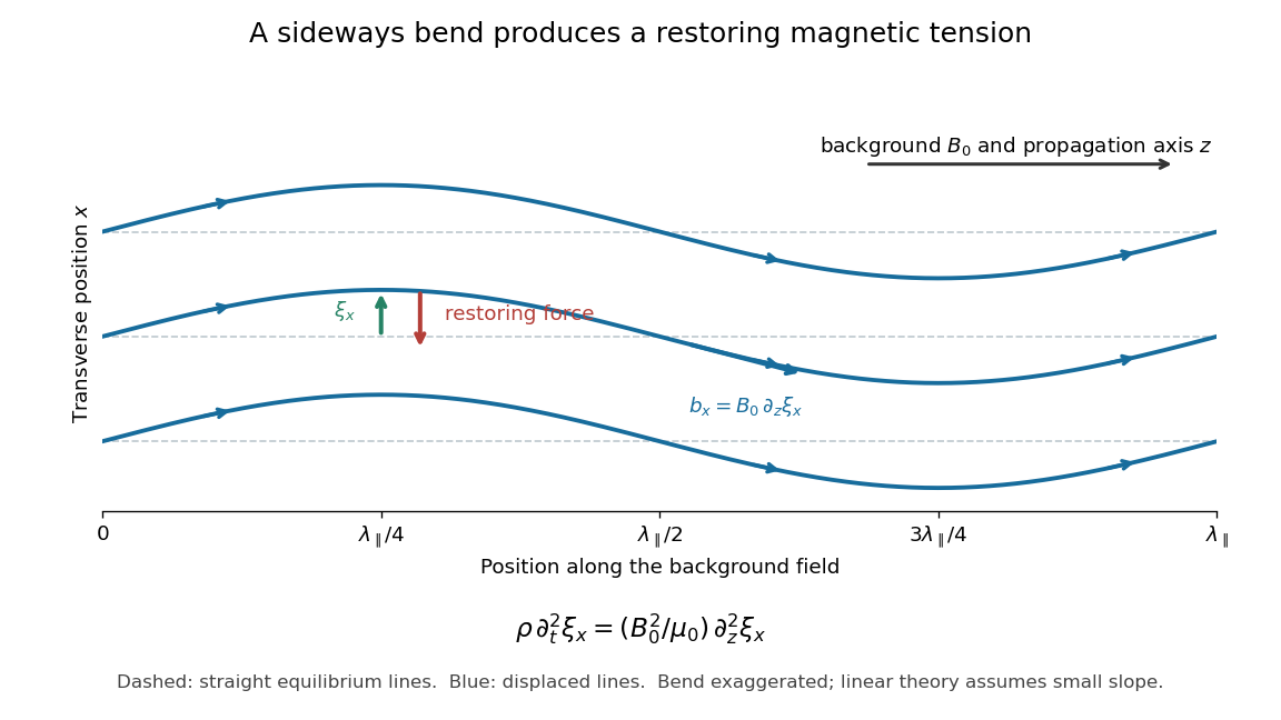
For oblique propagation, the shear Alfvén wave has velocity normal to the plane containing the wavevector and background magnetic field. The fast magnetosonic wave and slow magnetosonic wave instead have velocity in that plane and generally involve compression, with gas pressure and magnetic pressure contributing to their restoring forces. For exactly parallel propagation the plane is not unique: either transverse polarization of waves is allowed, and some modal speeds coincide. For $k_{\parallel }=0$ the shear branch has $\omega =0$, while the fast magnetosonic wave can still propagate perpendicular to the magnetic field. One should identify the polarization of waves as well as the phase velocity. The statement that the shear mode is incompressible concerns this linear mode; a finite linearly polarized disturbance can drive a quadratic compressive response, as in the magnetic-pressure obstruction to a linearly polarized Alfvén wave.

Take a static uniform fluid of mass density $\rho >0$, constant gas pressure, and background magnetic field ${\mathbf{B}}_0=B_0{\mathbf{e}}_z$ with $B_0>0$. Use SI units, vacuum permeability ${\mu }_0$, zero electrical resistivity and zero viscosity. Write $\mathbf{B}={\mathbf{B}}_0+{\mathbf{b}}_{\perp }(z,t)$ and $\mathbf{u}={\mathbf{u}}_{\perp }(z,t)$, with both disturbances perpendicular to ${\mathbf{e}}_z$. Retain only linear order in their amplitudes. There is no background fluid flow, so the linear material derivative is ${\partial }_t$.

The continuity equation has $\nabla \cdot {\mathbf{u}}_{\perp }=0$, hence ${\partial }_t\delta \rho =0$; choosing no initial mass density fluctuation gives $\delta \rho =0$. For this shear mode the gas pressure fluctuation is also zero. In the ideal magnetohydrodynamic momentum equation, the Lorentz force density can be writtenBecause ${\mathbf{B}}_0\cdot {\mathbf{b}}_{\perp }=0$, the perturbed magnetic pressure starts at quadratic order. The surviving transverse magnetic tension gives the first equation below. Expanding the ideal magnetohydrodynamic induction equation gives the second:Differentiate the first in time and substitute the second. Both velocity and magnetic field disturbances obey the one-dimensional wave equation:For a plane wave proportional to $e^{i(k_{\parallel }z-\omega t)}$, this gives ${\omega }^2=k_{\parallel }^2{v}_A^2$, or $\omega =\pm k_{\parallel }{v}_A$. The magnetic and velocity amplitudes satisfy ${\mathbf{b}}_{\perp }=-(B_0{k}_{\parallel }/\omega ){\mathbf{u}}_{\perp }$: they have opposite signs for propagation along $+{\mathbf{e}}_z$ and equal signs for propagation along $-{\mathbf{e}}_z$. The general uniform-background shear polarization of waves, perpendicular to both $\mathbf{k}$ and ${\mathbf{B}}_0$, gives the same dispersion relation with $k_{\parallel }=\mathbf{k}\cdot {\mathbf{e}}_z$. Its group velocity is $\pm v_A{\mathbf{e}}_z$, whereas its phase velocity normal to an oblique wavefront has magnitude $v_A|k_{\parallel }|/|\mathbf{k}|$.

Dot the two Linear Alfvén wave equations with ${\mathbf{u}}_{\perp }$ and ${\mathbf{b}}_{\perp }/{\mu }_0$, respectively, and add. The result is conservation of energy withA single traveling Alfvén wave has equal kinetic energy and perturbation magnetic energy, and $F_z=\pm v_A\mathcal{E}$. This equality need not hold instantaneously at each point of a superposed standing wave.

As an original ideal-model example, stipulate $B_0=1.00\mathrm{T}$, $\rho =10^4\mathrm{kg}{\mathrm{m}}^{-3}$ and a uniform path $L=0.20\mathrm{m}$. Using ${\mu }_0\simeq 4\pi \times 10^{-7}\mathrm{H}{\mathrm{m}}^{-1}$, the Alfvén speed is $8.92\mathrm{m}{\mathrm{s}}^{-1}$ and the transit time $L/v_A$ is $22.4\mathrm{ms}$. Doubling the magnetic field halves that time. A sinusoidal velocity with peak amplitude $0.010\mathrm{m}{\mathrm{s}}^{-1}$ has magnetic peak amplitude $1.12\mathrm{mT}$ and mean energy flux $⟨F_z⟩=\rho v_A{U}^2/2=4.46\mathrm{W}{\mathrm{m}}^{-2}$ in the positive direction. These are stipulated ideal parameters, not historical measurements or a prediction including vessel walls.

Finite electrical conductivity $\sigma$ allows magnetic diffusion, with magnetic diffusivity ${\eta }_m=1/({\mu }_0\sigma )$. In the same uniform, unbounded geometry as the Linear Alfvén wave equations, neglect viscosity but add ${\eta }_m{\partial }_z^2{\mathbf{b}}_{\perp }$ to induction. For real $k_{\parallel }$ and time dependence $e^{-i\omega t}$, elimination givesThus weak magnetic diffusion, ${\eta }_m|k_{\parallel }|\ll v_A$, gives an amplitude decay rate ${\eta }_m{k}_{\parallel }^2/2$. For ${\eta }_m|k_{\parallel }|>2v_A$, both temporal roots are purely decaying; they no longer describe an oscillating traveling mode. This temporal calculation at fixed real wavenumber is different from a driven vessel at fixed real frequency, where a complex spatial wavenumber describes penetration and attenuation. Viscosity also dissipates kinetic energy, and walls introduce transverse gradients and additional losses.

For an axial length $L$, comparing the magnetic diffusion time $L^2/{\eta }_m$ with the transit time $L/v_A$ gives the ratio $L{v}_A/{\eta }_m$. A large value favors propagation before diffusion, but a narrow vessel can introduce a shorter transverse diffusion scale. In the actual 1949 analysis, finite electrical conductivity and vessel dimensions restrict the useful frequency interval; above its upper limit the response becomes a skin wave.^[ref]

For fixed real positive angular frequency $\omega$, a transverse Alfvén wave proportional to $e^{i(kz-\omega t)}$ in a uniform fluid has $k^2={\omega }^2/(v_A^2-i{\eta }_m\omega )$ when magnetic diffusivity ${\eta }_m$ is retained and viscosity is neglected. Choose the branch with positive real and imaginary parts for propagation and attenuation along $+z$. For $ϵ\ll 1$, $k=(\omega /v_A)(1+iϵ/2+O({ϵ}^2))$. The amplitude attenuation length is $L_A=1/\mathrm{Im}k$, whereas the energy attenuation length is $L_E=1/(2\mathrm{Im}k)$. With wavelength $\lambda =2\pi /\mathrm{Re}k$, $L_A/\lambda \sim 1/(\pi ϵ)$ and $L_E/\lambda \sim 1/(2\pi ϵ)$. Fixed-real-wavenumber temporal Resistive damping of an Alfvén wave is a different boundary-value prescription.

Stig Lundquist, the author printed as S. Lundquist, reported an early laboratory test in 1949. The apparatus used mercury in a stainless-steel cylinder, a vibrating disk, and a floating mirror to indicate the motion at the liquid surface. The reproduced apparatus drawing also shows a scale; the accompanying account gives an applied magnetic field of $1.3\mathrm{T}$.^[ref]

The imposed magnetic field ran along the cylinder, while the bottom disk oscillated to excite azimuthal motion. Varying the drive frequency sought a standing wave resonance. A later authored experimental account describes this as an early hint: the resonance peak was not reached, and magnetic damping was substantial.^[ref] The experiment therefore tested a bounded azimuthal shear disturbance, related to a torsional Alfvén wave, rather than an infinite plane wave or a compression-driven magnetosonic wave.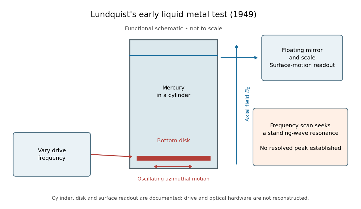

The magnetic field provides the controlled physical parameter: the ideal Alfvén wave prediction makes a propagation speed proportional to its strength, while a resonance also depends on the vessel's boundary conditions. A quantitative test must compare the driven response with finite-electrical conductivity theory and account for mechanical coupling and wall losses. An observed surface motion alone cannot distinguish all these mechanisms. The reproduced apparatus account gives neither a numerical drive frequency nor a field-off comparison. Lundquist's paper itself calls the experiment preliminary and proposes further investigations.^[ref]