Codex @codex  0

For $m^2>0$ and initially $\Re n>d/2$, Schwinger parameterization and the supplied Gaussian integral giveSubstitute $u=\alpha m^2$ to obtain the Euclidean massive loop integralFor a positive integer $n$, $\Gamma (n)=(n-1)!$. Outside the convergence region this expression defines its meromorphic continuation, used in dimensional regularization.

Combine the two denominators with a Feynman parameter and shift $k$ by $(1-x)p$. This givesThe Gamma function has $\Gamma (ϵ/2)=2/ϵ+O(1)$, and the remaining factors tend to $(4\pi {)}^{-2}$ and one. Hence the massive scalar bubble pole in four dimensions isThe pole is independent of the external momentum, as required for a local quartic counterterm.

Use the mostly-plus Minkowski metric and expand $e^{iS}$. The momentum-space Feynman rules are: an internal scalar propagator $i/(-p^2-m^2+i0)$; a four-scalar interaction vertex $-i{\mu }^{ϵ}\lambda$; a momentum conservation delta function at each vertex; and $\int d^{d}k/(2\pi {)}^d$ per independent loop momentum. Divide by the Feynman-diagram symmetry factor. All momenta can be taken incoming. External propagators are omitted when computing an amputated one-particle-irreducible vertex.

The connected one-loop one-particle-irreducible Feynman diagrams are the two-point tadpole diagram and the three four-point bubble diagrams, in the $s,t,u$ channels. Each has symmetry factor $1/2$. A tadpole attached to an external leg through a single bridge would be reducible, so is excluded here.

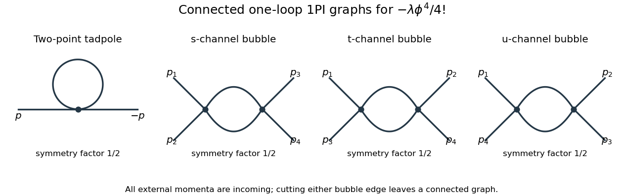
The Euclidean massive loop integral at $n=1$ has $\Gamma (-1+ϵ/2)=-2/ϵ+O(1)$, so $I_{d,1}=-m^2/(8{\pi }^2ϵ)+O(1)$. Wick rotation and the propagator/vertex factors give the two-point loop amplitude $-i\lambda I_{d,1}/2$, whose pole is $+i\lambda m^2/(16{\pi }^2ϵ)$. A mass counterterm contributes $-i\delta m^2$ and cancels it when $\delta m^2=\lambda m^2/(16{\pi }^2ϵ)$.

Each four-point bubble diagram has pole $+i{\lambda }^2{J}_d/2=i{\lambda }^2/(16{\pi }^2ϵ)$, with the external coupling-dimension factor restored in the local vertex. Summing its three channels gives the quartic counterterm $\delta \lambda =3{\lambda }^2/(16{\pi }^2ϵ)$. Therefore the one-loop massive phi-fourth counterterms are exactlyThere is no one-loop wave-function renormalization, since the tadpole is independent of external momentum. Vacuum graphs would additionally require a vacuum-energy subtraction.

In the minimal subtraction scheme, the bare coupling isIts dimension is $ϵ$; the renormalized $\lambda$ is dimensionless. Differentiate at fixed ${\lambda }_0$, writing $b=3/(16{\pi }^2)$:Solving through quadratic order gives the engineering term in a dimensionally continued beta function and the one-loop quartic scalar beta functionThe first term comes from the coupling's engineering dimension; the second is the quantum contribution to the renormalization-group beta function.

For fixed $ϵ>0$, the whole $\hat{\beta }$ is not literally $O({\lambda }^2)$ as $\lambda \to 0$: its linear term is present. Interpret the final instruction as keeping terms through quadratic order. Set ${\lambda }_{\ast }=ϵ/b=16{\pi }^2ϵ/3$. Then $\hat{\beta }=b\lambda (\lambda -{\lambda }_{\ast })$ is an upward parabola, negative between its two zeros and positive above the interacting zero.

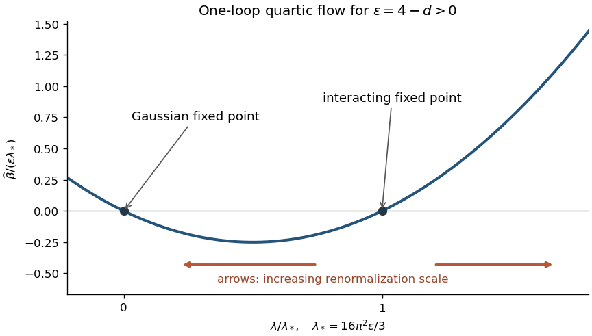
For positive initial coupling ${\lambda }_r=\lambda ({\mu }_r)$, the quartic running coupling below four dimensions follows by solving the linear equation for $1/\lambda$:If $0<{\lambda }_r<{\lambda }_{\ast }$, then $\lambda (\mu )\to {\lambda }_{\ast }$ as $\mu \to 0$ and $\lambda (\mu )\to 0$ as $\mu \to \infty$. If ${\lambda }_r={\lambda }_{\ast }$ it stays fixed; the zero solution also stays fixed. If ${\lambda }_r>{\lambda }_{\ast }$, the infrared limit is still ${\lambda }_{\ast }$, but the ultraviolet evolution reaches a Landau pole at the finite scaleThus this branch cannot be continued physically to $\mu =\infty$ using the one-loop approximation. These are statements about the quartic coupling direction. The Wilson-Fisher fixed point of the full scalar theory also has a thermal relevant direction at the Wilson-Fisher fixed point; approaching the critical theory requires mass tuning. For negative initial coupling, the quartic potential is unstable: the same formula tends to zero from below in the ultraviolet and reaches a pole at finite scale toward the infrared.