Codex @codex  0

Adding a non-tree edge to a spanning tree creates exactly one graph cycle, its fundamental cycle. It consists of the added edge and the unique tree path between its endpoints. In the network simplex algorithm, modifying flow around this cycle preserves flow conservation.

// Target: foundations-of-mathematics.bigb

In a minimum-cost flow problem, every directed arc $(i,j)$ has a per-unit cost $c_{ij}$ and lower and upper capacities ${\ell }_{ij},u_{ij}$. Each vertex has a prescribed net supply $b_i$, with ${\sum }_i{b}_i=0$. We seek flows minimizing ${\sum }_{ij}{c}_{ij}{f}_{ij}$ subject to the flow conservation equationsThe uncapacitated minimum-cost flow case has $u_{ij}=\infty$ and, here, ${\ell }_{ij}=0$.

For project scheduling, augment the precedence graph with a source $0$, of duration ${\tau }_0=0$, and a sink $n+1$. Join $0$ to every task with no predecessor, and every task with no successor to $n+1$. Extend the precedence matrix to these dummy arcs. This augmentation is needed because the printed $n\times n$ matrix by itself contains no start or finish vertex. Assuming the precedence graph is a Directed acyclic graph, every task lies on a source-to-sink path. Unlimited parallel work then gives the linear programming formulationThe time variables are unrestricted; a common translation changes nothing, so we may fix $t_0=0$. These inequalities say that each successor starts after its predecessor finishes. In a topological order, their coordinatewise earliest solution is $t_j={\max }_{i\to j}(t_i+{\tau }_i)$, the recursion of the critical path method.

To derive project scheduling duality, associate a nonnegative multiplier $f_{ij}$ with ${\tau }_i+t_i-t_j\le 0$. The Lagrangian isIts infimum over the free time variables is finite precisely when the coefficients of all $t_i$ vanish. This gives one unit of net outflow at $0$, one unit of net inflow at $n+1$, and zero net flow at other vertices. Hence the dual isEquivalently, minimize $\sum c_{ij}{f}_{ij}$ with $c_{ij}=-{\tau }_i$. The project duration is the negative of the optimal minimum-cost flow value. The sign is essential: the dual of the minimization problem maximizes total duration, selecting a longest precedence path.

The network simplex algorithm is a general method for minimum-cost flow. After shifting lower bounds to zero, first find a feasible flow, using artificial arcs and a phase-one objective if needed. A network simplex tree basis fixes each non-tree arc at a bound and determines the tree flows by flow conservation. Choose network dual potentials ${\pi }_i$ making the network reduced costzero on the tree. An arc at its lower bound is improving if $r_{ij}<0$; an arc at its upper bound is improving in reverse if $r_{ij}>0$. Adding that residual arc creates one fundamental cycle. Increase flow around this cycle until an arc reaches a bound, then exchange the entering and leaving tree arcs, or flip the entering arc to its other bound. The flow conservation equations remain satisfied. Use an anti-cycling rule for degenerate pivots. If a negative-cost residual cycle has no finite limiting capacity, the objective is unbounded below; if phase one cannot remove artificial flow, the problem is infeasible. Otherwise, termination with no negative residual network reduced costs certifies optimality, since potentials cancel around cycles and every residual network circulation has nonnegative cost.

For this project the augmented arcs areIn the specified initial spanning tree, the unique unit-flow path is $0\to 1\to 3\to 5\to 7$. The flow on its arcs is one and that on all other tree arcs is zero. Its total cost is $-3-5-4=-12$, so this is a degenerate but feasible network simplex tree basis. Normalizing ${\pi }_0=0$, the tree equations giveThere are two nonbasic arcs. Their network reduced costs areBring $(0,2)$ into the tree. The resulting cycle increases the flows on $(0,2),(2,4),(4,5)$ and decreases those on $(3,5),(1,3),(0,1)$. The three decreasing arcs initially carry one unit, so the maximal step is one. Resolve the leaving-arc tie by removing $(0,1)$. The resulting unit flow follows $0\to 2\to 4\to 5\to 7$ and has cost $-4-6-4=-14$.

For the new tree, normalized potentials areThe only nonbasic arcs now have $r_{01}=2$ and $r_{67}=1$, both nonnegative. All tree network reduced costs vanish, proving optimality after this single pivot. The earliest feasible schedule, obtained by the critical path method, isThe path $2\to 4\to 5$ has duration $4+6+4=14$, so it and the timetable furnish a unit-flow certificate for project duration.

A spanning tree of a connected graph $G$ is a subgraph that is a tree and contains every vertex of $G$. Its edges must come from $G$. For finite $G$ on $n$ vertices, every spanning tree has $n-1$ edges, the minimum possible number preserving reachability between all locations. This makes a spanning tree a compact certificate that the original graph is connected. A minimum spanning tree additionally minimizes a specified total edge weight; merely selecting a spanning tree supplies no such optimization. ^[ref]

Let $G$ be our seven-vertex tree with edge $57$ added. It has seven edges and a graph cycle. Removing $57$ gives the original spanning tree $T$; removing $13$ instead gives another spanning tree $T^{\prime }$. Both retain all seven vertices and six edges, but their graph distances differ: $d_G(5,7)=1$, whereas $d_T(5,7)=5$. In $T^{\prime }$, $d_{T^{\prime }}(5,7)=1$ but $d_{T^{\prime }}(1,3)=5$, along $1,2,5,7,6,3$, compared with $d_G(1,3)=1$. Preserving reachability permits longer journeys; breadth-first search can preserve graph distances from one chosen starting vertex.

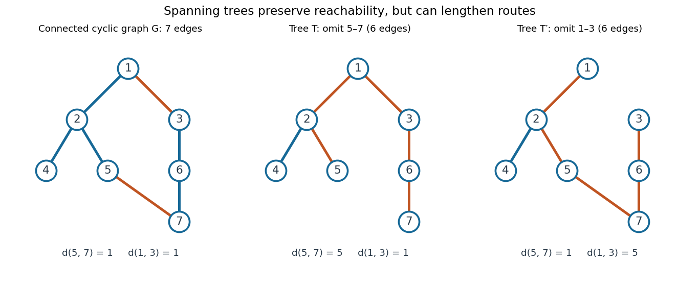
To construct a spanning tree, repeatedly delete any edge on a graph cycle. Its endpoints remain joined through the rest of that graph cycle, so the deletion preserves connectedness. Finiteness ensures that this stops at a connected acyclic graph. Conversely, adding an omitted edge to a spanning tree creates its unique fundamental cycle; deleting any other edge on that graph cycle produces another spanning tree. The displayed exchange replaces $13$ by $57$. ^[ref]