Gaussian instrument broadening in third-order pulse correlation is the widening produced when an ideal third-order intensity autocorrelation is convolved with an additional Gaussian instrument response. It is a model of the measurement, not a universal correction for every correlator. The finite width of the optical nonlinear gate is already part of the ideal third-order trace and must not be counted again as an independent response.
Let a Gaussian pulse have intensity standard deviation . Its ideal trace is a Gaussian with . Take the additional normalized impulse response to beThe convolution isThe response preserves integrated trace area while reducing peak height and increasing variance. Since every Gaussian full width at half maximum has the same conversion factor from standard deviation,
For an original example, and give an ideal correlation width about and a measured width about . The peak falls to approximately 0.853 of the ideal peak under this unit-area response. Dividing the measured width only by would overestimate the pulse duration.
The correct Gaussian inversion is when the radicand is positive. Its conditioning worsens near the response floor: the derivatives with respect to and are and . Small width errors can therefore cause large errors in a narrowly resolved pulse. Gaussian pulse-width deconvolution uncertainty must include uncertainty of the characterized response, with covariance if relevant.
The primary correlator used second-harmonic generation, sum-frequency generation, crossed beams and spatial imaging to encode delay. It did not assert that every additional broadening mechanism was a Gaussian convolution.[ref]
A Single Shot 3rd Order Cross-Correlator for Pulse Contrast and Pulse Shape Measurements by J. Collier and others. printed pp. 194–195, third-order integral, Description and Figure 2
To apply this model, characterize the response under the same optical alignment, spectral acceptance and detector conditions. Non-Gaussian wings, clipping or unresolved side lobes require a different model; a smaller sampling step cannot by itself remove optical broadening.Gaussian pulse-width deconvolution uncertainty is the uncertainty in an inferred pulse duration after subtracting a characterized Gaussian instrument contribution. For the Gaussian instrument broadening in third-order pulse correlation model, let be measured correlation full width at half maximum, the additional response width and the inferred pulse width:These widths must use the same convention. The relation already includes the ideal nonlinear gate; represents an additional response.
First-order propagation uses the sensitivity coefficientsThus the standard uncertainty obeysThe negative covariance term follows from the subtraction, not a rule that uncertainties should simply be subtracted. The GUM's general law retains covariance and requires considering higher-order terms when nonlinearity is significant.[ref]
Guide to the expression of uncertainty in measurement by JCGM. §§5.1.2–5.1.3 and 5.2, sensitivity coefficients, nonlinear limitation and correlated inputs
For an original example, and give . With independent , the formula gives . If instead the two width estimates have correlation coefficient 0.8 with those same uncertainties, the covariance is and . The assumed relationship between the estimates changes the result.
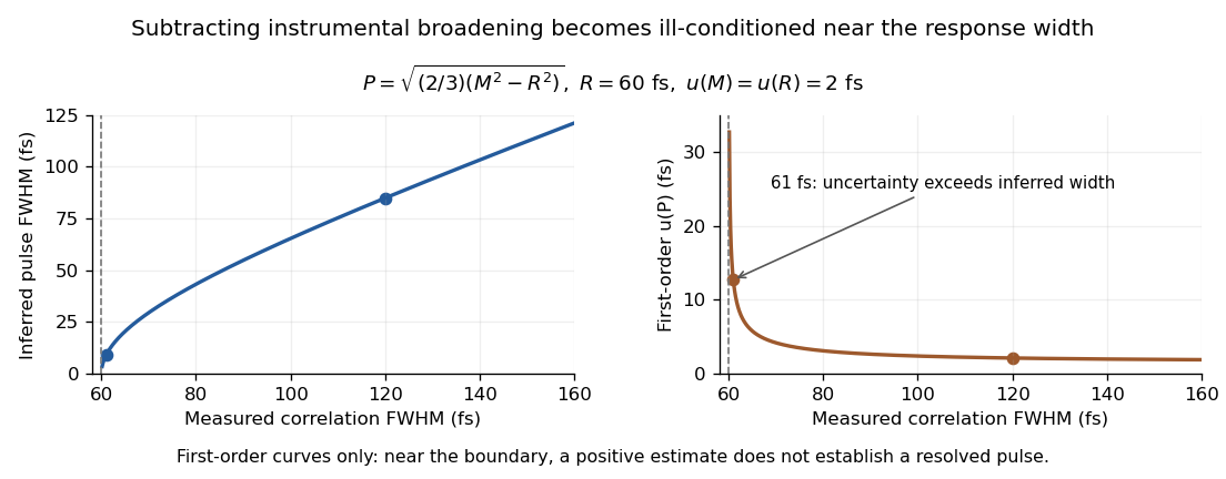
Original Gaussian pulse-width inversion and first-order uncertainty curves for a 60 fs response and independent 2 fs width uncertainties
. Details. 
Near , both derivatives grow because approaches zero. With , and independent 2 fs uncertainties, the central inferred value is only about while the first-order uncertainty is about . This is an unresolved Gaussian pulse-width estimate under these measurement conditions, rather than a reliably resolved 9 fs pulse.
The quantity being subtracted is , with approximate variance . If plausible width values include , linear symmetric error bars on can be misleading. Report the response assumptions and consider an appropriate nonlinear inference or bound; simply discarding negative radicands would silently change the statistical model. Even a precise inversion remains conditional on the Gaussian response model being physically appropriate.
An unresolved Gaussian pulse-width estimate occurs when the measured correlation width and characterized response do not establish a positive pulse width with useful precision under the assumed Gaussian model. It is a limitation of the measurement and inference, not evidence that the pulse has zero duration.
In Gaussian pulse-width deconvolution uncertainty, the inferred full width at half maximum isFor , a positive central value exists. Whether the data resolve it depends on the uncertainty in , the response model and their covariance, not just on the sign of the central radicand.
Take original central values and . They give and . Independent standard uncertainties give, to first order,This uncertainty is almost three times the central difference. Propagating once more through the square root gives ; that symmetric approximation is poorly suited to the boundary . The GUM requires attention to higher-order terms when nonlinearity invalidates the first-order approximation.[ref]
Guide to the expression of uncertainty in measurement by JCGM. §5.1.2, nonlinear functions and higher-order terms; §5.2, covariance
A simple range calculation makes the difficulty visible without assigning a probability. Suppose only that plausible widths lie in and . These ranges include equal widths, hence , while their maximum positive radicand is , giving . These stipulated ranges are not a calibrated confidence interval; they demonstrate sensitivity to response uncertainty.
A negative observed need not imply an imaginary physical duration: noise, incorrect response characterization or a non-Gaussian pulse can invalidate the naive inversion. Conversely, dropping all negative simulated radicands and averaging the rest conditions on a selected subset and biases the inference. A Monte Carlo method must implement a stated input or likelihood model and a justified treatment of the physical boundary.
Report the measured and response widths, their conventions, uncertainties and dependence. An upper limit is meaningful only with its statistical construction and coverage assumptions. Improved response characterization or an independent temporal measurement can resolve the ambiguity; quoting more digits of the positive square root cannot.
Articles by others on the same topic
There are currently no matching articles.