An optical pulse is a finite-duration envelope of light. A nearly monochromatic pulse has many carrier oscillations within its duration : in units with light speed one, its wavelength obeys . A slowly varying propagation-time map stretches the pulse duration by its derivative and divides the observed frequency by the same factor.
// Target: general-relativity.bigb
An optical postpulse is a secondary optical pulse arriving after the chosen main pulse. Specify the delay, relative peak radiant power, duration and collected laser pulse energy: a relative peak alone does not determine the energy of a differently shaped replica. It is distinct from an extended optical pulse pedestal and from electronic ringing from a photodetector.
A transparent plate provides a concrete mechanism. At normal incidence, a transmitted replica that makes one additional internal round trip has approximate delaywhere is plate thickness and is its group refractive index. Neglect absorption, dispersion and overlap, and let each internal reflection retain power fraction . The first delayed replica then has approximately times the directly transmitted energy. This etalon round-trip delay can create a physical optical echo.
For an original chosen , and , the delay is about and the energy ratio is . A main pulse would be followed by a replica under that model. The historical single-shot correlator experiment deliberately inserted a BK7 etalon to generate and detect such a delayed pulse.[ref]
A Single Shot 3rd Order Cross-Correlator for Pulse Contrast and Pulse Shape Measurements by J. Collier and others. printedp195, Results and Figure4, double-reflection postpulse near1.5×10^-3
Changing the plate thickness tests the delay prediction; changing optical alignment tests whether a stray reflection is involved. A third-order intensity autocorrelation can distinguish temporal sides under its model, while a symmetric second-order intensity autocorrelation cannot alone assign a feature to a prepulse or postpulse. An opposite-delay correlation feature may instead be a third-order pulse correlation ghost; it need not identify another physical pulse.
An etalon round-trip delay is the extra envelope travel time associated with one additional internal round trip in an etalon. At normal incidence, for a transparent plate of thickness and a sufficiently narrowband optical pulse,The relevant quantity is group refractive index, since the delay concerns the pulse envelope. The extra propagation phase is ; its derivative gives . This assumes negligible frequency-dependent reflection phase and treats dispersion locally.
For an original chosen plate with and , the delay is about . A pulse transmitted after one extra round trip appears that much later than the directly transmitted pulse. Another extra round trip adds the same delay in this local model, producing an echo sequence. The optical postpulse article separately describes the reflection losses that determine echo energies.
The frequency-domain connection gives an independent consistency check. Neighboring transmission resonances differ in round-trip phase by , so the local free spectral range satisfiesThe example predicts about . This etalon delay inferred from free spectral range uses the same local dispersion assumptions; the spacing can vary across a broad spectrum.
The historical third-order correlator calibrated its delay coordinate by inserting a BK7 etalon of known thickness into an arm and measuring the trace shift.[ref]
A Single Shot 3rd Order Cross-Correlator for Pulse Contrast and Pulse Shape Measurements by J. Collier and others. printed p. 195, Description, group-delay calibration; Results and Figure 4, delayed replica
A plate inserted into an arm also changes the direct propagation delay relative to the displaced air path; that single-pass insertion delay is distinct from the echo's extra internal round trip. Oblique incidence, dispersive coatings and broad-band pulse reshaping require a more complete propagation model.An etalon round-trip phase is the phase accumulated by a circulating optical field after one complete internal round trip, relative to its earlier passage. At normal incidence through a uniform plate of thickness ,where the last terms are the phases of the two internal amplitude-reflection coefficients. Propagation and reflection both contribute; a coating phase is not automatically zero.
The resonance condition follows from a field sum. If , with , successive transmitted paths contain factors . Their geometric series has denominator . Its squared magnitude containsFor slowly varying amplitudes, transmission peaks occur near . The primary manufacturer tutorial describes the resulting etalon transmission peaks and distinguishes their spacing from their width.[ref]
A constant phase offset shifts resonance positions without changing the local slope. In an original model with constant round-trip delay , adding reflection phase shifts a given resonance by approximately . The free spectral range remains in this constant-slope model.
Frequency-dependent phase has a different effect. Differentiating with respect to angular frequency givesThe last two terms form an etalon coating group delay. A stipulated propagation contribution plus coating contribution gives local resonance spacing about , rather than 50 GHz. These are illustrative phase functions, not measured coating specifications.
Use a continuous branch of wave phase when differentiating: jumps of in a wrapped display are not physical delay spikes. The etalon delay inferred from free spectral range article derives the interval relation between phase slope and adjacent resonances. Finite pulse bandwidth, angular spread and frequency-dependent reflection amplitudes determine how closely the simple resonance model describes an actual optical pulse.
An etalon coating group delay is the frequency derivative of the reflection phase contributed by the two coatings during one internal round trip. At fixed incidence and polarization, write the internal reflection coefficients as . With the phase convention of etalon round-trip phase,The phases must refer to consistently chosen surfaces: moving a reference plane transfers a propagation contribution between the terms. Only the consistently defined total is directly comparable with the resonance spacing.
A constant coating phase changes the positions of resonances but contributes zero group delay. A linear phase produces constant group delay. Curvature produces group delay dispersion:A highly reflecting coating therefore cannot be characterized by reflectance alone. The manufacturer's ultrafast-mirror documentation separately specifies reflection dispersion and shows multiple-bounce arrangements for compensation.[ref]
Chirped Mirrors by Thorlabs. Dispersion-Compensating Mirrors, phase/GD/GDD characterization and Fig. 1.1
For an original constant-slope example, suppose propagation contributes and the coatings together contribute . The local free spectral range is approximately , rather than . Ignoring coating delay would overassign that to propagation when inferring a spacer thickness or group index. The values are stipulated, not a coating specification.
For an independent curvature example, let the summed coating phase contain , with . Across a frequency interval , its group delay changes by . The derivative is with respect to angular frequency; omitting changes the result.
Experimentally, one may measure adjacent resonance frequencies and compare their spacing with an independently characterized spacer and group index. A discrepancy alone cannot uniquely identify coating delay: spacer dispersion, incidence angle and geometry also affect the result. Etalon delay inferred from free spectral range gives an interval-averaged phase slope; identifying it with a single-frequency derivative requires sufficiently slow variation. The simple manufacturer's spacer relation explicitly neglects spacer dispersion.[ref]
Etalon Tutorial by Iridian Spectral Technologies. Free Spectral Range section and displayed plate relation
Etalon reference-plane dependence is the change in the assigned propagation and reflection phases when the mathematical planes defining an etalon's field amplitudes are moved. A consistently computed etalon round-trip phase and its resonance frequencies remain unchanged. The decomposition into spacer delay and etalon coating group delay depends on those planes.
Use time dependence and a lossless uniform spacer with wavenumber . Let the physical interfaces be separated by , with internal reflection coefficients referred to their surfaces. The round-trip multiplier isThe multilayer formalism explicitly assigns forward and backward amplitudes at specified interfaces and propagates their phases through each layer. Its sign conventions must remain consistent when comparing reflection phases.[ref]
Multilayer optical calculations by Steven J. Byrnes. §4.1, interface amplitudes and propagation; Appendix A, reflection-amplitude conventions
Move the left mathematical reference plane a distance into the spacer, leaving the actual coating in place. A wave launched from that plane travels to the coating and back, so the effective left reflection coefficient becomes . The explicit remaining distance is . HenceThis original derivation changes the representation, not the physical cavity. Moving a real mirror would instead change the system.
Let , using continuous wave phase. Since , the new assigned terms obeyTheir sum equals . If the spacer is dispersive, the corresponding second-derivative contributions likewise transfer between the two terms; the total group delay dispersion is unchanged.
For an original example, take and . The assigned reflection delay increases by about while the assigned propagation delay decreases by the same amount. The free spectral range cannot reveal a change of bookkeeping. An apparent discrepancy of that size between two coating calculations can arise solely from different reference planes.
Report the incident medium, polarization, reference surfaces and phase convention with a coating-delay result. A measured resonance spectrum constrains the total phase; independently identifying a coating contribution requires a compatible spacer model. Etalon delay inferred from free spectral range therefore should not be compared with an isolated coating derivative until both calculations use the same reference planes.
An etalon delay inferred from free spectral range estimates an etalon round-trip delay from the frequency spacing of adjacent transmission resonances. When round-trip group delay varies little across that spacing,The measured quantity is resonance spacing, not the width of one resonance. The manufacturer tutorial explicitly distinguishes free spectral range from optical finesse, which compares that spacing with an individual peak's width.[ref]
The relation follows from wave phase. Let be the total etalon round-trip phase, including relevant reflection phases. Adjacent resonances satisfy . Defining gives the exact interval relationThus the reciprocal spacing is the delay averaged over that frequency interval. Interpreting it as a local pulse-envelope delay requires sufficiently weak variation across the interval and relevant pulse spectrum.
For a uniform plate at normal incidence with negligible frequency-dependent reflection phase, . Differentiation gives , where is the group refractive index. Treating as frequency independent recovers the manufacturer tutorial's elementary plate formula; using a phase index in a strongly dispersive material can instead give the wrong delay.
An original measured-spacing example takes . The inferred delay is . A spacing standard uncertainty of contributes approximately to the delay uncertainty through . With stipulated and negligible coating delay, the corresponding plate thickness is about .
In a spectral experiment, identify adjacent peaks of the same resonance family and calibrate the frequency coordinate. If the coordinate is wavelength, use rather than treating a wavelength interval as a frequency interval. Beam angle, dispersion and reflection phase belong in the propagation model.
A time-domain check looks for replicas separated by the predicted extra round trip. The historical single-shot correlator experiment inserted a known-thickness BK7 etalon to calibrate delay and separately placed an uncoated etalon in the input to create a double-reflection postpulse.[ref]
A Single Shot 3rd Order Cross-Correlator for Pulse Contrast and Pulse Shape Measurements by J. Collier and others. printed p. 195, Description, Results and Figure 4
The single-pass delay caused by inserting glass into an arm is distinct from the additional round-trip separation of successive transmitted replicas.An optical prepulse is a secondary optical pulse arriving before the reference main pulse. The sign of its delay is part of the definition: choose the main pulse at , so a prepulse has negative arrival time. A weak earlier pulse and an equally weak optical postpulse can affect a target differently when the material retains a response to the earlier illumination. Temporal order therefore carries information that one total laser pulse energy does not.
An original separated rectangular-profile example uses a main pulse of duration and a prepulse of duration centred earlier. Let the prepulse's peak radiant power be of the main peak. The optical pulse temporal contrast is , but the energy ratio isThus the prepulse carries of the two-pulse energy. If the main pulse carries , the prepulse carries . These stipulated disjoint power profiles have no field-overlap term, and the main pulse's full width at half maximum does not reveal the earlier contribution.
A temporal diagnostic needs both sufficient delay coverage and calibrated dynamic range. The single-shot third-order correlator paper motivates its asymmetric response by contrasting it with the symmetric second-order trace, which loses the distinction between before and after.[ref]
A Single Shot 3rd Order Cross-Correlator for Pulse Contrast and Pulse Shape Measurements by J. Collier and others. printedp194, Introduction and Figure1
Its delay axis still needs a known physical reference. A third-order pulse correlation ghost from a real postpulse can appear on the prepulse side; interpreting every small lobe as earlier light would be incorrect.Repeating the measurement while varying an independently characterized optical delay helps assign temporal order. Record the detector baseline subtraction, coverage and response width along with the trace. A nondetection means a limit within those measurement conditions, rather than proof of zero early optical energy.
An optical pulse pedestal is lower-level optical power extending around a pulse's dominant short peak. It can precede the peak, follow it or extend on both sides. A broad pedestal can carry substantial laser pulse energy while barely changing the peak's full width at half maximum. Optical pulse temporal contrast describes the relative power levels; integrated energy also depends on how long each contribution persists.
For an original power-profile model, choose a central rectangular contribution of height and duration , together with a pedestal of height and duration , centred at the same time. Let . The peak power is , while the pedestal lies below half of that value. The power FWHM is therefore still , butThese are stipulated additive power contributions, not a rule for adding coherent electric fields.
Set and . The pedestal then contains half the total energy even though its power is about a thousand times below the main peak. With and , each contribution carries . The peak-to-pedestal power ratio is exactly in this example. An inverse convention would quote a small pedestal-to-peak ratio instead; state which contrast definition is being used.
A measurement needs temporal range as well as dynamic range. A narrow scan can miss broad wings, while a readout that resolves only the peak can bury a pedestal in its own background. A commercial example is the Sequoia third-order cross-correlation instrument, whose manufacturer identifies temporal-contrast measurement as its purpose and separately specifies scan range and temporal resolution.[ref]
Sequoia temporal contrast measurement by Amplitude. PDF pp. 1–2, measurement purpose, third-order cross-correlator, scan and resolution specifications
The cited instrument description establishes the measurement approach; the numerical profile above is an independent model.A real optical pedestal must also be distinguished from detector baseline subtraction errors. Blocked-beam and reference measurements characterize the detector background, while a suitable optical measurement tests whether low-level light accompanies the pulse. A detection time gate that excludes a pedestal changes the admitted energy relative to a detector integrating the full waveform.
The pedestal energy fraction is the fraction of an optical pulse's laser pulse energy assigned to its optical pulse pedestal. Specify the decomposition and integration interval before quoting it. For a nonnegative additive radiant power model ,The assumptions imply by integration. A pedestal fit is a model of the measured radiant power; it is not automatically a unique physical separation into optical fields. Overlapping fields with optical coherence can have wave interference terms, so their separate field energies cannot generally be added as though those terms were absent.
The distinction from optical pulse temporal contrast is quantitative. Use the stipulated rectangular model of optical pulse pedestal: a main contribution has height and duration , while a centered pedestal has height and duration . For , the total peak is and the power full width at half maximum remains . Define peak-to-pedestal contrast . ThenHalf the laser pulse energy is in the modeled pedestal when . A large peak-to-pedestal ratio therefore does not by itself imply a small energy contribution.
For an original comparison, fix and the same in both traces. With , the pedestal fraction is ; with , it is . Thus the same contrast and power FWHM can coexist with about1% or50% pedestal energy. At fixed finite , increasing the pedestal duration can make approach one without changing that FWHM.
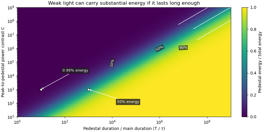
Optical energy outside a time gate is a related observable that avoids assigning a pedestal underneath the main peak. For a specified gate containing that peak,In the rectangular example with equal to the main interval, . At and , this is , while . The difference is pedestal power inside the gate, which the outside-gate measurement does not label separately.
The analysis must also specify its temporal coverage and detector baseline subtraction. Subtracting actual weak light as though it were detector background changes the inferred laser pulse energy. A short detection time gate omits outlying light instead. Neither operation is justified solely by knowing the peak-to-pedestal contrast. The Sequoia technical sheet illustrates why temporal coverage and resolving power are separate instrument properties: it lists scan range, scan resolution and optical temporal resolution independently.[ref]
Sequoia temporal contrast measurement by Amplitude. January2024 sheet, PDFp2, Specifications
Optical energy outside a time gate is the radiant energy excluded by a specified ideal temporal acceptance set . For a nonnegative radiant power profile of finite positive total energy,The time-integral definition is the radiometric one.[ref]
International Lighting Vocabulary by CIE. entry17-21-041, note1, radiant energy as the integral of radiant flux
This observable needs a gate boundary but no fitted separation into a main field and an optical pulse pedestal.For an original three-pulse example, let an optical prepulse, main pulse and optical postpulse carry , and respectively, with disjoint supports. A gate containing only the main pulse admits of , so . Widening that gate to include the postpulse reduces the fraction to . The optical waveform has not changed; the admitted observable has.
For a translated interval with continuous boundary values,Unequal power at the boundaries produces first-order sensitivity to a timing shift. Equal boundary values eliminate this derivative but need not eliminate higher-order loss; quadratic energy loss from centred Gaussian gate timing error gives an existing example.
The total-energy denominator must cover the excluded light too. If the acquisition window misses an unknown tail, pulse-energy interval from incomplete tail measurements supplies conditional bounds rather than an exactly known fraction. A detection time gate on an electrical detector trace also includes the detector impulse response and is not automatically an ideal gate on incoming optical power. A characterized optical response and a stated detector baseline subtraction are needed to compare the two.
Optical pulse temporal contrast compares a pulse's peak with weaker light at another time. For a radiant power trace with peak , explicitly choose either the peak-to-local ratio or its inverse . The first is at least one where the local power is positive; the second lies between zero and one. With a fixed transverse beam shape, the same ratio can be formed from light intensity. If the beam shape changes with time, specify the spatial sampling instead of identifying local intensity and total power.
A plateau at of the peak has and . Expressing this power ratio as optical contrast in decibels givesFor an amplitude ratio whose power ratio is , the same definition gives . Contrast also needs a delay or time range: an optical prepulse, an optical postpulse and a long optical pulse pedestal can have the same relative height but different positions and laser pulse energies. The pedestal energy fraction additionally requires integration over the contribution's duration.
A useful nonlinear measurement is third-order intensity autocorrelation. In an ideal instantaneous model, an input light intensity generates a second-harmonic gate proportional to . Sum-frequency generation with a delayed fundamental replica gives a recorded signal proportional toThe instrument measures this cross-correlation, rather than simply reading . Finite gate width, phase matching, spatial overlap and detector response enter the interpretation.
The1998/99 instrument of J. Collier and colleagues used second-harmonic generation, a Wollaston prism and an optical biprism to form crossing fundamental and harmonic beams. A second crystal generated the sum-frequency signal, imaged through optical filters onto a charge-coupled device. Position encoded delay. An inserted glass etalon produced a delayed replica near of the main signal, recorded on one side of the correlation peak. Figure4 combines window settings shifted with etalons.[ref]
A Single Shot 3rd Order Cross-Correlator for Pulse Contrast and Pulse Shape Measurements by J. Collier and others. Printedpp194–195, Description/Figure2 and Results/Figure4
An independent ideal calculation explains both the asymmetry and a possible third-order pulse correlation ghost. Let represent two identical-shape pulses with well-separated supports and correlation lobes, with the second weaker and delayed. Squaring introduces no overlap term. If , expansion givesThe delayed replica produces a lobe of relative order , while the opposite-delay ghost has order . For , the scales are about and respectively. These values are predictions of the stated ideal model. Assigning every small correlation feature directly to a separate input pulse would miss this distinction.
A nondetection below the measurement floor establishes a bound under a detection model, rather than demonstrating that no light exists there. Finite dynamic range, detector baseline subtraction, delay coverage and resolution should accompany a reported contrast trace. The Sequoia manufacturer likewise distinguishes optical temporal resolution from the scan step; making that step smaller does not alone narrow the optical response.[ref]
Sequoia temporal contrast measurement by Amplitude. January2024 sheet, PDFp2, Specifications
Optical contrast in decibels expresses a specified ratio logarithmically. For peak-to-local radiant power contrast ,The inverse convention gives . State the convention and the time of the weak feature. A peak-to-feature contrast means one million to one in power, not in field amplitude.
An original readout example uses a linear photodetector whose baseline-corrected output is proportional to optical power. A main reading of and weak-feature reading of imply and . Applying to those readings would incorrectly report : the electrical signal represents power, not optical wave amplitude.
If instead a measurement is proportional to an optical field amplitude , with the same impedance and spatial normalization for both fields, power is proportional to . ThenA field-amplitude ratio of and a power ratio of therefore express the same contrast. The correct multiplier follows the measurement model, not whether the readout unit happens to be volts.
Contrast does not specify pedestal energy fraction, optical prepulse duration or delay coverage. The Sequoia primary sheet specifies dynamic range, scan range and optical temporal resolution separately.[ref]
Sequoia temporal contrast measurement by Amplitude. January2024 technical sheet, PDFp2, Specifications
A signal beneath a known measurement floor supports a contrast bound within that window; subtracting an uncertain background does not establish unlimited contrast.An energy-normalized pulse profile separates an optical pulse's temporal shape from its total laser pulse energy. For nonnegative radiant power and finite , define . Then has units inverse time and integrates to one. The radiant energy in a time interval is times the integral of over that interval.[ref]
International Lighting Vocabulary by CIE. Entry17-21-041, note1, radiant energy as integrated radiant flux
For an original two-lobe example, let during and during , with zero values elsewhere. The two integrals are and . Choosing gives powers and , and energies and . Multiplying by two doubles both powers without changing .
The temporal energy centroid of an optical pulse is when this moment exists. Here it is , in the gap between lobes. An energy centroid need not be a location of maximum power.
Mathematically, is a probability density function, but its weighting here is energy over time. It is not automatically a measured photon-arrival distribution, particularly when photon energies vary. A zero-energy trace cannot be normalized this way, and a noisy baseline-corrected trace with negative excursions is not automatically a nonnegative density. The Gaussian pulse energy and peak power article gives one normalized shape family.
The temporal energy centroid of an optical pulse is its energy-weighted mean time. For nonnegative radiant power with finite positive energy and finite absolute first moment,The normalization uses radiant energy as integrated radiant flux.[ref]
International Lighting Vocabulary by CIE. entry 17-21-041, note 1
The centroid is a moment of the energy-normalized pulse profile; it need not coincide with the largest power value, a threshold crossing or the middle of the FWHM interval.For an original two-component example, let ninety percent of the energy belong to a symmetric narrow component centred at zero and ten percent to a symmetric component centred at . Linearity of the integral gives . Weak delayed energy can move the centroid even when the dominant peak remains near zero. Multiplying the whole power trace by a positive constant leaves unchanged; translating it by shifts its centroid by .
A detector response can shift the measured centroid too. Suppose a normalized impulse response and normalized optical profile have finite absolute first moments. For their convolution , direct integration with givesThus a causal exponential detector response of time constant shifts the recorded centroid by in this model. NIST's pulsed-radiometer characterization explicitly measures detector impulse responses and uses convolution to assess reproduced waveforms.[ref]
Calibration Service for Low-level Pulsed-Laser Radiometers at 1.06 µm: Pulse Energy and Peak Power by Rodney W. Leonhardt. §§6.1–6.2, printed pp. 13–15
The centroid identity is the independent moment calculation above.Baseline drift can cause a separate shift. Suppose a true pulse has and , but a positive residual baseline of remains across the analysis window from to . Its added energy is , centred at . The resulting centroid isA waveform measurement should therefore record the time window, baseline estimate and detector timing response with its reported centroid. A negative background-subtracted trace also needs care: it is not automatically a nonnegative energy distribution.
A flying focus is an optical pulse whose position of maximum focusing varies with time because different frequencies focus at different axial locations and arrive at different times. For a broad incident Gaussian beam, and spectral phase give and , hence . This is the velocity of a focusing pattern, which can exceed or be negative without individual portions of the field propagating faster than light.
The carrier-envelope phase locates the carrier oscillation relative to the envelope of an optical pulse. In with envelope maximum at zero, it is the displayed phase modulo . Few-cycle dynamics can depend on it even when cycle-averaged light intensity is unchanged. A pulse train's phase increment is related to its carrier-envelope offset frequency; signs depend on the complex-field convention.
Measure the spectrum of a nonlinear optical gate signal as its relative delay is varied. A retrieval algorithm seeks a complex pulse consistent with the resulting two-dimensional intensity record and the particular gate law. Different gate laws have different ambiguities and response limitations; a small fitting residual alone does not guarantee stable pulses or correct calibration.
An optical Kerr gate rotates a probe's polarization in proportion to a delayed replica's intensity in the weak-gate regime. Resolving the gated spectrum gives a pulse-characterization record with a third-order gate law, distinct from a second-harmonic gate.
The self-gated second-harmonic spectrogram has the displayed ideal form. Its delay marginal is proportional to the intensity autocorrelation by the Parseval identity. Absolute time and wave phase are undetermined; and also give the same record. Finite crystal acceptance and spatial walk-off modify the ideal gate.
A Gaussian pulse has a field or intensity envelope specified by a Gaussian function; the distinction must be stated. For the displayed intensity, the temporal full width at half maximum is . A transform-limited pulse with this shape has intensity spectral and temporal widths satisfying . A quadratic spectral phase can lengthen the pulse without changing its spectral intensity.
The Gaussian pulse field-envelope width is the full width at half maximum of the magnitude of a Gaussian electric-field envelope. It differs from the FWHM of radiant power. For a fixed spatial mode with and constant ,The Gaussian pulse energy and peak power article derives this relation. Power-FWHM is also the convention explicitly used for PULSELENGTH in the primary source documentation.[ref]
Plane wave and beam source - Simulation object in Ansys Optics documentation. Standard source, PULSELENGTH definition and manual time-signal calculation
For an original example, a power width of corresponds to field-envelope width . At the field-envelope half-maximum points, the power is one quarter of its peak, since . At the power half-maximum points, the field magnitude is instead of its peak. A threshold applied to one measured quantity therefore does not define the other quantity's FWHM.
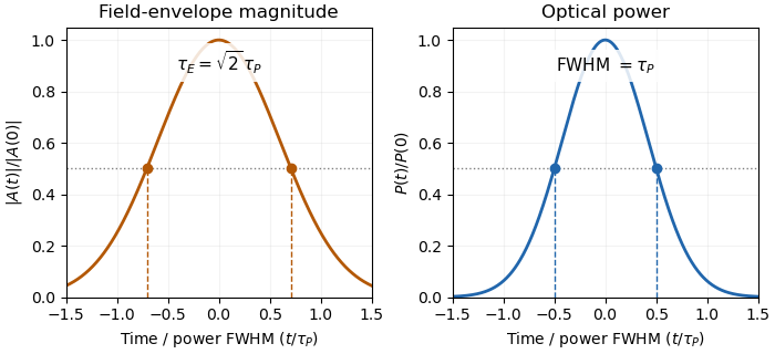
Squaring a Gaussian field envelope narrows its full width at half maximum by a factor of square root two.
Details. The envelope magnitude is distinct from the rapidly oscillating signed electric field. A direct photodetector generally supplies a power-related electrical trace, further modified by its impulse response; it is not a direct recording of the optical carrier's field envelope. Inserting an amplitude width into a power-width peak power formula consequently uses the wrong convention. State the observable and the response model with the reported pulse duration.
The Gaussian pulse time-gate energy fraction is the share of an isolated pulse's laser pulse energy admitted by a finite time window. The result below acts on incident optical radiant power. Let be the power full width at half maximum, and first place the pulse centre and the detection time gate centre at zero.
A detection time gate need not collect the whole pulse. Integrating the same profile only over gives the Gaussian pulse time-gate energy fractionwhere is the error function. A gate as wide as the power full width at half maximum collects only , or 76.10% of the pulse energy. The pulse has nonzero Gaussian tails outside that interval. A real readout's impulse response can extend the required integration window further.
Alignment adds a parameter. Let the pulse centre be , the gate centre be , and write the Gaussian gate centring error as . Put . Integrating the normalized Gaussian pulse profile over the gate givesAt the two error function terms reduce to the centred formula above. With and , the captured fraction drops to . The pulse centre then lies on a gate edge. Merely keeping the gate width fixed does not keep its collected energy fixed.
The gate works best when centred. With the centred energy-normalized pulse profile and , differentiation of givesA Gaussian function is an even function about its centre and decreases with distance from that centre. Thus for , and symmetry gives the opposite sign for . The same argument proves that a centred interval maximizes mass for an even unimodal density; unimodality supplies the required monotonicity.
A centred gate of width captures of the energy. Solving gives for 99% capture in this ideal model. The requirement changes if the centring error is nonzero.
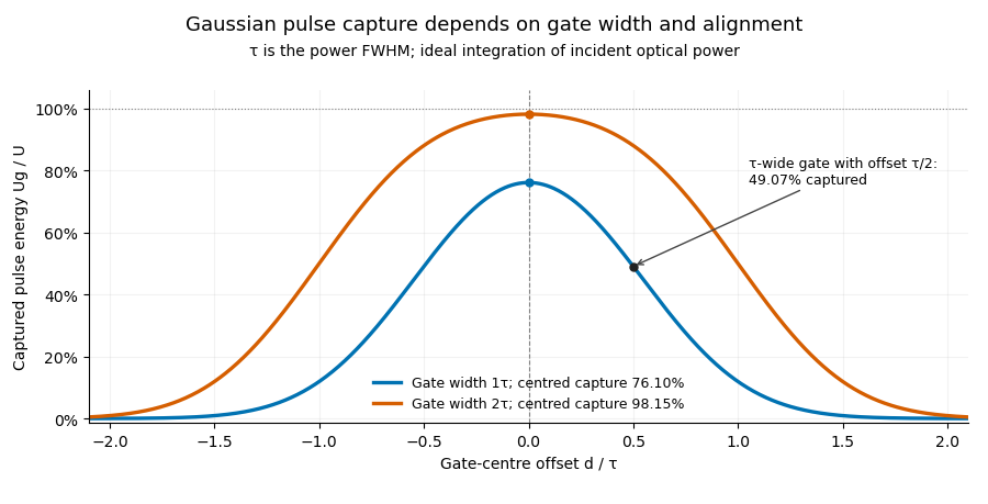


Pulse timing jitter can therefore create variation in gated energy even when every full pulse has the same . A wider gate reduces this loss but also changes admitted background and the chance of including neighbouring pulses. Measure the timing and detector response associated with the chosen gate.
For a detector modeled as a linear time-invariant system, its recorded waveform is a convolution of the optical input with its impulse response. NIST tested avalanche photodiode radiometers with roughly optical pulses, recorded their responses with an oscilloscope, and convolved measured responses with longer Gaussian inputs to estimate corrections. The detector and amplifier were characterized together.[ref]
Calibration Service for Low-level Pulsed-Laser Radiometers at 1.06 µm: Pulse Energy and Peak Power by Rodney W. Leonhardt. §§6.1–6.2, printed pp. 13–15: short-pulse excitation, sampling readout and numerical convolution
A gate applied to that electrical waveform must use the readout model rather than assuming the optical fraction is unchanged.The Gaussian gate centring error is , the time displacement between a gate centre and a Gaussian pulse centre. The Gaussian pulse time-gate energy fraction gives the full displaced-gate formula. Equal positive and negative errors collect equal energy in that symmetric model, so an energy deficit alone does not reveal the direction of the misalignment.
A focused expansion explains sensitivity close to the optimum. Let be the centred energy-normalized pulse profile, let , and define . For the Gaussian standard deviation ,Thus the leading quadratic energy loss from centred Gaussian gate timing error is second order, rather than linear in .
For an original example, take a gate as wide as the power FWHM . Its centred fraction is . An error gives from the full formula; the quadratic approximation gives . For this is a displacement, with gate width and total pulse energy unchanged.
A delay scan of a gated readout can locate the maximum, provided the source and gate widths remain stable. Pulse timing jitter produces a distribution of offsets rather than a single deterministic . Also distinguish a gate on optical power from one on a detector's electrical waveform: NIST measured detector impulse responses and used convolution to assess pulse reproduction.[ref]
Calibration Service for Low-level Pulsed-Laser Radiometers at 1.06 µm: Pulse Energy and Peak Power by Rodney W. Leonhardt. §§6.1–6.2, short-pulse response measurement and numerical convolution
Quadratic energy loss from centred Gaussian gate timing error is the leading decrease in collected energy when a symmetric gate is displaced slightly from the centre of a Gaussian pulse. At the optimum the first-order change vanishes, but the second-order change is negative. The Gaussian pulse time-gate energy fraction gives the exact displaced-gate integral; here the local loss and its effect on jitter are derived explicitly.
Let be the centred energy-normalized pulse profile, let , and setThe Leibniz integral rule gives . Since is even and ,The Taylor expansion therefore yieldsThis is an absolute fraction of the full pulse energy. The relative loss compared with the centred gate is instead .
For a gate as wide as the power FWHM , and . An offset gives leading loss , or about percent of the centred gate's collected energy. Neither the full pulse energy nor the gate width has changed.
A zero mean offset does not eliminate this loss. For a sufficiently narrow random offset with mean and variance , the leading expectation isIf has a centred normal distribution, the quadratic model also gives . At , the leading mean loss is and this standard deviation is . These formulas neglect fourth-order effects; they are local approximations, not bounds for large timing excursions.
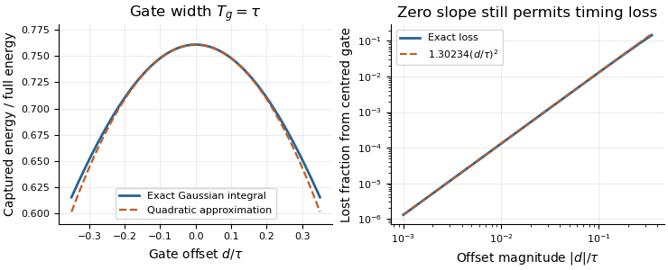
Exact Gaussian gate capture and its local quadratic loss: a zero first derivative does not remove timing sensitivity.
Details. 
An apparatus check scans the gate delay about its optimum and compares the measured decrease with the model, while monitoring gate width and the pulse. A gate on the detector's electrical output need not act directly on optical power: the detector impulse response and readout convolution must be included. NIST's impulse-response measurements illustrate that distinction.[ref]
For an isolated Gaussian pulse, the relation between laser pulse energy and peak power depends on the pulse-width convention. Here is the total incident radiant power, the background is zero, and denotes the power full width at half maximum. Integrating over the entire pulse defines its positive energy .
Pulse energy, peak power and average power resolve different information. Consider a Gaussian pulse withThe chosen pulse duration is the full width at half maximum of radiant power: . It refers to radiant power, rather than the wave amplitude of the electric field. The Gaussian integral gives the relation between Gaussian pulse energy and peak power:The pulse energy shape factor is . It equals for this power profile; a rectangular pulse of duration has . Knowing only a width and an integrated energy therefore requires a pulse-shape assumption before inferring peak power.
An equivalent form makes the normalization transparent. Write the pulse centre as , and let denote the standard deviation of its energy-normalized pulse profile:The ratio is a probability density function in the mathematical sense: it is nonnegative, has units , and integrates to one. Here it weights the pulse's energy over time. Its normal distribution profile has mean and variance . This gives without a separate area estimate.
For a stipulated and , the power full width at half maximum is and the peak power is . Confusing the standard deviation with the full width at half maximum would insert the wrong duration into the conversion.
The Gaussian pulse field-envelope width is a second distinct convention. If a fixed spatial field profile gives for a constant , the wave amplitude envelope obeysConsequently its amplitude full width at half maximum is . Inserting into the formula for a power-width input underestimates the true peak power by a factor . State which measured waveform defines the width.
An electrical photodetector trace can also be broadened by its impulse response. The optical pulse-width inference therefore needs a characterized detector response.[ref]
The product of a specified temporal width and spectral frequency width. State whether each width refers to power or field amplitude and whether it is a full width at half maximum or a standard deviation.
A transform-limited pulse needs coherent phases across its contributing frequency range. A laser's usable gain bandwidth therefore sets a duration scale through the time-bandwidth product, as displayed. The wavelength interval must first be converted to frequency; the simple conversion is only a narrow-band approximation. Numerical constants depend on pulse shape and width convention: a Gaussian intensity envelope has . A hard gain interval is not automatically a spectral FWHM. Mode locking can arrange the longitudinal modes' phases, while group velocity dispersion must be controlled to approach the transform limit. The cavity round-trip time sets pulse spacing, rather than this bandwidth-limited width.
A diagnostic proportional to for delay . It does not uniquely reconstruct a complex optical electric field; extracting pulse duration requires a shape model.
A third-order intensity autocorrelation measures the delay-dependent intensity productThe name counts three intensity factors. A physical implementation can use two second-order nonlinear processes: second-harmonic generation creates a gate proportional to , and sum-frequency generation mixes it with a delayed fundamental replica. It therefore need not use a third-order material susceptibility. The historical device spatially encoded delay in crossing beams and imaged the sum-frequency signal onto a charge-coupled device.[ref]
A Single Shot 3rd Order Cross-Correlator for Pulse Contrast and Pulse Shape Measurements by J. Collier and others. printedpp194–195, equation forA3, Description and Figure2
An original Gaussian calculation illustrates response width. Set . Completing the square in the integral givesHence the third-order correlation width of a Gaussian pulse obeys for intensity full widths at half maximum. A correlation width would imply within this ideal Gaussian model. The square-root-of-two conversion appropriate to second-order Gaussian intensity autocorrelation would be different.
For a general pulse, need not equal ; this asymmetry can distinguish a delayed feature from an earlier one. It is still a cross-correlation with a finite-width nonlinear gate, rather than a direct reading of . The existing optical pulse temporal contrast derivation shows how a delayed weak replica also produces an opposite-delay third-order pulse correlation ghost.
Characterize phase matching, beam overlap, spatial uniformity and the temporal response before interpreting a narrow feature. Scaling the input intensity by scales this ideal signal by , so input fluctuations also matter. The measured trace does not uniquely reconstruct an arbitrary complex optical electric field.
The third-order correlation width of a Gaussian pulse converts a measured ideal third-order intensity autocorrelation width to the width of its assumed Gaussian intensity profile. If the pulse intensity has temporal standard deviation , its squared intensity gate has deviation . Their cross-correlation haswhere both values are intensity full widths at half maximum. The parent third-order intensity autocorrelation article derives the complete Gaussian trace by integration. The factor concerns that shape family and that correlation definition; it is not a universal pulse-width conversion.
A focused extension separates a known instrument response. Suppose an additional normalized Gaussian response of width convolves the ideal trace. Addition of Gaussian variances givesFor an original chosen and , the inferred pulse width is . Applying only the ideal conversion would give . This Gaussian instrument broadening in third-order pulse correlation assumes that the additional response really acts as a Gaussian convolution; it is not an empirical correction for every correlator.
The historical physical implementation used second-harmonic generation followed by sum-frequency generation and spatial delay encoding.[ref]
A Single Shot 3rd Order Cross-Correlator for Pulse Contrast and Pulse Shape Measurements by J. Collier and others. printed pp. 194–195, equation for A3 and Description/Figure 2
Optical gate width, phase matching and spatial overlap belong to its response model. A finer scan step alone does not demonstrate a smaller optical response width.If the assumed response width equals or exceeds the measured width, the displayed subtraction does not provide a resolved positive pulse width. Non-Gaussian traces, satellites and chirped fields also require explicit modeling; an intensity-width conversion does not reconstruct the optical wave phase.
Gaussian instrument broadening in third-order pulse correlation is the widening produced when an ideal third-order intensity autocorrelation is convolved with an additional Gaussian instrument response. It is a model of the measurement, not a universal correction for every correlator. The finite width of the optical nonlinear gate is already part of the ideal third-order trace and must not be counted again as an independent response.
Let a Gaussian pulse have intensity standard deviation . Its ideal trace is a Gaussian with . Take the additional normalized impulse response to beThe convolution isThe response preserves integrated trace area while reducing peak height and increasing variance. Since every Gaussian full width at half maximum has the same conversion factor from standard deviation,
For an original example, and give an ideal correlation width about and a measured width about . The peak falls to approximately 0.853 of the ideal peak under this unit-area response. Dividing the measured width only by would overestimate the pulse duration.
The correct Gaussian inversion is when the radicand is positive. Its conditioning worsens near the response floor: the derivatives with respect to and are and . Small width errors can therefore cause large errors in a narrowly resolved pulse. Gaussian pulse-width deconvolution uncertainty must include uncertainty of the characterized response, with covariance if relevant.
The primary correlator used second-harmonic generation, sum-frequency generation, crossed beams and spatial imaging to encode delay. It did not assert that every additional broadening mechanism was a Gaussian convolution.[ref]
A Single Shot 3rd Order Cross-Correlator for Pulse Contrast and Pulse Shape Measurements by J. Collier and others. printed pp. 194–195, third-order integral, Description and Figure 2
To apply this model, characterize the response under the same optical alignment, spectral acceptance and detector conditions. Non-Gaussian wings, clipping or unresolved side lobes require a different model; a smaller sampling step cannot by itself remove optical broadening.Gaussian pulse-width deconvolution uncertainty is the uncertainty in an inferred pulse duration after subtracting a characterized Gaussian instrument contribution. For the Gaussian instrument broadening in third-order pulse correlation model, let be measured correlation full width at half maximum, the additional response width and the inferred pulse width:These widths must use the same convention. The relation already includes the ideal nonlinear gate; represents an additional response.
First-order propagation uses the sensitivity coefficientsThus the standard uncertainty obeysThe negative covariance term follows from the subtraction, not a rule that uncertainties should simply be subtracted. The GUM's general law retains covariance and requires considering higher-order terms when nonlinearity is significant.[ref]
Guide to the expression of uncertainty in measurement by JCGM. §§5.1.2–5.1.3 and 5.2, sensitivity coefficients, nonlinear limitation and correlated inputs
For an original example, and give . With independent , the formula gives . If instead the two width estimates have correlation coefficient 0.8 with those same uncertainties, the covariance is and . The assumed relationship between the estimates changes the result.
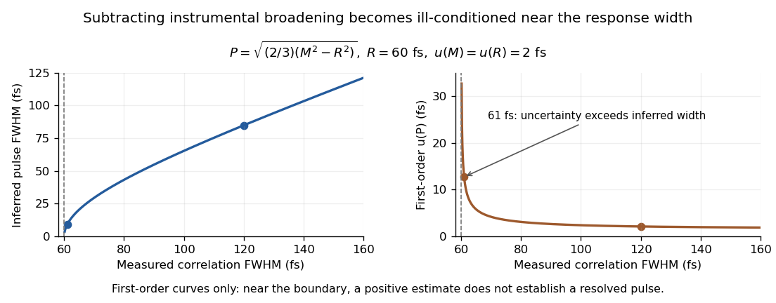
Original Gaussian pulse-width inversion and first-order uncertainty curves for a 60 fs response and independent 2 fs width uncertainties
. Details. 
Near , both derivatives grow because approaches zero. With , and independent 2 fs uncertainties, the central inferred value is only about while the first-order uncertainty is about . This is an unresolved Gaussian pulse-width estimate under these measurement conditions, rather than a reliably resolved 9 fs pulse.
The quantity being subtracted is , with approximate variance . If plausible width values include , linear symmetric error bars on can be misleading. Report the response assumptions and consider an appropriate nonlinear inference or bound; simply discarding negative radicands would silently change the statistical model. Even a precise inversion remains conditional on the Gaussian response model being physically appropriate.
An unresolved Gaussian pulse-width estimate occurs when the measured correlation width and characterized response do not establish a positive pulse width with useful precision under the assumed Gaussian model. It is a limitation of the measurement and inference, not evidence that the pulse has zero duration.
In Gaussian pulse-width deconvolution uncertainty, the inferred full width at half maximum isFor , a positive central value exists. Whether the data resolve it depends on the uncertainty in , the response model and their covariance, not just on the sign of the central radicand.
Take original central values and . They give and . Independent standard uncertainties give, to first order,This uncertainty is almost three times the central difference. Propagating once more through the square root gives ; that symmetric approximation is poorly suited to the boundary . The GUM requires attention to higher-order terms when nonlinearity invalidates the first-order approximation.[ref]
Guide to the expression of uncertainty in measurement by JCGM. §5.1.2, nonlinear functions and higher-order terms; §5.2, covariance
A simple range calculation makes the difficulty visible without assigning a probability. Suppose only that plausible widths lie in and . These ranges include equal widths, hence , while their maximum positive radicand is , giving . These stipulated ranges are not a calibrated confidence interval; they demonstrate sensitivity to response uncertainty.
A negative observed need not imply an imaginary physical duration: noise, incorrect response characterization or a non-Gaussian pulse can invalidate the naive inversion. Conversely, dropping all negative simulated radicands and averaging the rest conditions on a selected subset and biases the inference. A Monte Carlo method must implement a stated input or likelihood model and a justified treatment of the physical boundary.
Report the measured and response widths, their conventions, uncertainties and dependence. An upper limit is meaningful only with its statistical construction and coverage assumptions. Improved response characterization or an independent temporal measurement can resolve the ambiguity; quoting more digits of the positive square root cannot.
A third-order pulse correlation ghost is a correlation lobe generated by a real feature in the nonlinear gate, appearing at a delay where no separate input pulse need exist. It is a property of the measurement's cross-correlation, not automatically an optical prepulse or optical postpulse.
The optical pulse temporal contrast article derives the separated-replica model for , and nonoverlapping identical-shape pulses. In third-order intensity autocorrelation, the main, positive-delay and opposite-delay lobe weights are respectivelyThe physical delayed replica enters linearly when it meets the strong squared gate; its squared contribution to the gate creates the opposite-delay ghost. Lobe separation and negligible pulse overlap are assumptions of this simple decomposition.
For an original , the real postpulse has four percent of the main intensity and equal duration. Normalized to the correlation's main peak, its lobe is , while the ghost is . A feature at negative delay near that latter level does not establish a physical prepulse. The ghost-to-real-lobe ratio is exactly in this model. This ghost-level consistency test for a delayed pulse replica can check an interpretation, although an actual prepulse could also be present.
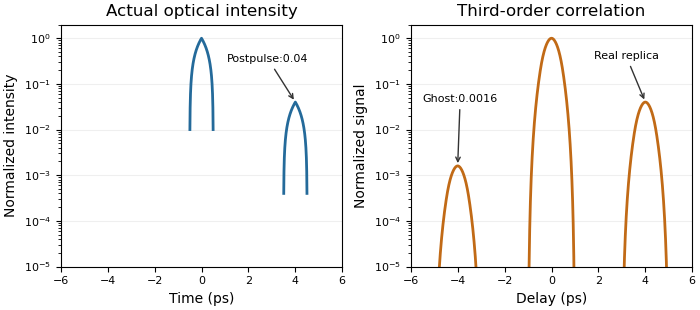
A real optical postpulse creates an opposite-delay ghost in an ideal third-order intensity autocorrelation
. Original compact triangular intensity profiles with a delayed replica at4ps and relative peak0.04. Direct numerical correlation produces the opposite-delay lobe near0.0016; the optical profile has no pulse there. Each panel is normalized to its own maximum. Source. Details.
The historical correlator's inserted-etalon test supplies a controlled physical postpulse for checking the delay orientation.[ref]
A Single Shot 3rd Order Cross-Correlator for Pulse Contrast and Pulse Shape Measurements by J. Collier and others. printedp195, Results and Figure4
Independent changes to the replica strength, or a reference with known temporal structure, test the ghost interpretation. Overlapping pulses, unequal shapes and instrument backgrounds require a richer model.A ghost-level consistency test for a delayed pulse replica checks whether measured side lobes agree with the simple model of one real delayed pulse and its nonlinear correlation ghost. It can reject that model; agreement alone does not prove that no real prepulse exists.
Use the separated, identical-shape replica model in third-order pulse correlation ghost. Let be the positive-delay lobe and the opposite-delay lobe, each divided by the central correlation peak. For delayed-to-main intensity ratio ,Thus the measured ratio gives , and the first equation supplies an additional consistency condition. The frequently useful approximation omits the small central-peak correction; exactly, .
For an original pair of measured relative heights and , their ratio would require . That value predicts , not . These two readings therefore cannot both come from the stated single-replica model with equal instrument sensitivity at the two delays. A real earlier pulse is one possible explanation, but background, unequal pulse shapes or additional replicas can also invalidate the model.
An independent check varies the delayed replica while holding the main pulse fixed. Before central-peak normalization, halving halves the real side lobe and quarters its ghost. This attenuation scaling of a third-order correlation ghost probes the nonlinear origin rather than only one accidental height match. The existing parent diagram shows a direct numerical example without an actual pulse at the ghost's delay.
The historical correlator's inserted-etalon experiment provided a controlled physical postpulse and a known temporal direction.[ref]
A Single Shot 3rd Order Cross-Correlator for Pulse Contrast and Pulse Shape Measurements by J. Collier and others. printed p. 195, Results and Figure 4
The algebraic height test here is an independent ideal calculation. Use unsaturated, background-corrected readings with comparable response and lobe resolution; otherwise the measured ratios need not represent the model's intensities.Attenuation scaling of a third-order correlation ghost tests the nonlinear origin of a side lobe by changing a real delayed replica's strength while preserving the main pulse. The diagnostic prediction differs from attenuating the entire input. The quantity attenuated must be stated as an intensity or energy ratio, rather than confused with a field-amplitude ratio.
Use the nonoverlapping equal-shape model , with and . Let an independently controlled intensity transmission act on the delayed replica only. With the main pulse fixed, the third-order intensity autocorrelation has central, real-replica and third-order pulse correlation ghost lobe weights proportional toThe common factor is the same single-pulse correlation amplitude. Thus the real lobe has logarithmic slope 1 and its ghost slope 2 versus replica transmission, before normalization. Their exact ratio is .
An original example starts with . Initially the weights are . Halving the delayed replica's intensity gives . The real side lobe halves while its ghost quarters. If each trace is divided by its own central peak, the predictions becomeThese normalized curves have the small additional central-peak dependence; treating them as exact pure powers would omit it.
In contrast, common attenuation in third-order pulse correlation sends for the complete two-pulse input. All three factors in acquire the same scaling, so every unnormalized lobe scales as . Halving the entire input therefore reduces every lobe eightfold while leaving the normalized shape unchanged. That experiment cannot demonstrate selective quadratic ghost scaling.
A suitable controlled test forms a delayed replica in a separate optical path, varies that path's transmission without changing its shape or delay, then recombines it with a monitored main pulse. Retain background-corrected, unsaturated readings and verify comparable detector response at both delays. The historical experiment's inserted-etalon postpulse supplied a physical delayed reference, not this particular attenuation sweep.[ref]
A Single Shot 3rd Order Cross-Correlator for Pulse Contrast and Pulse Shape Measurements by J. Collier and others. printed p. 195, Results and Figure 4, etalon-generated postpulse; printed p. 194, defining third-order integral
Agreement with the scaling model supports the ghost interpretation under its assumptions. It does not exclude an additional real optical prepulse, unequal replica shapes, overlapping fields or an attenuation-dependent background. Those possibilities require further independent observations.
Common attenuation in third-order pulse correlation multiplies the entire input intensity profile by one constant factor before the correlation is formed. For the ideal signalreplacing by gives . All unnormalized lobes scale together, so division by the central peak removes this common factor. The primary correlator paper defines the three-intensity-factor integral and implements it through second-harmonic generation and sum-frequency generation.[ref]
A Single Shot 3rd Order Cross-Correlator for Pulse Contrast and Pulse Shape Measurements by J. Collier and others. printed p. 194, defining integral and nonlinear optical implementation
The factor is an intensity transmission. An optical field-amplitude factor instead gives intensity factor and correlation factor . Confusing these conventions changes the predicted power law. A spectral filter that reshapes or chirps the pulse is also not necessarily a common scalar attenuation.
An original example takes an ideal central signal 100 and a side lobe 1 in consistent detector-signal units. Halving the full input intensity gives central 12.5 and side 0.125; their ratio remains 0.01. In contrast, attenuation scaling of a third-order correlation ghost changes only the delayed replica and predicts different real-lobe and ghost powers. A common attenuator cannot perform that selective test.
A fixed background changes what normalization appears to show. Add one unremoved signal unit to both locations. Before attenuation the observed side/center ratio is . After common intensity transmission , it is . The apparent side feature has grown relative to the peak even though the optical profile did not change. Detector baseline subtraction and a verified linear readout are therefore part of the experiment.
Shot-to-shot intensity variation supplies another consequence. Let the common intensity multiplier be , where has zero mean. ThenFor equally likely multipliers 0.9 and 1.1, the mean intensity is unchanged but the mean cubic signal is times the unit-intensity signal. This cubic intensity-noise bias in pulse correlation shows why cubing a mean input is not equivalent to averaging third-order signals. The calculation assumes the pulse shape is unchanged on each shot.
A controlled check records pulse intensity alongside the correlator signal, varies a broadband common attenuator, and tests cubic scaling in an unsaturated interval after background correction. Failure of that test can indicate detector nonlinearity, pulse reshaping or an uncontrolled background; it does not uniquely identify a particular fault. The ideal law applies only while the nonlinear gate and optical overlap retain their stipulated response.
Cubic intensity-noise bias in pulse correlation is the difference between the average of a third-order signal and the signal predicted from the average intensity when a fluctuating common intensity multiplier is cubed. Assume every shot has the same pulse shape, , with nonnegative scalar . The ideal third-order integral givesThe three intensity factors follow from the second-harmonic generation and sum-frequency generation gate.[ref]
A Single Shot 3rd Order Cross-Correlator for Pulse Contrast and Pulse Shape Measurements by J. Collier and others. printed p. 194, third-order correlation integral and apparatus
Let , with , variance and third central moment . Expanding the cube givesFor , write the coefficient of variation as and, when , skewness as . The relative multiplier is . For zero variance the multiplier is one without needing to define skewness.
Equally likely and have mean one and give mean cubic multiplier . Rare bright shots can matter much more: stipulated probabilities 0.9 and 0.1 at and also give mean one, butThe extra signal need not mean that the mean input intensity increased. These are original probability examples, not measurements reported in the correlator paper.
For unchanged pulse shape, common fluctuations multiply every delay by the same expected factor. Normalizing the averaged trace by its peak cancels that factor. Shape changes correlated with brightness destroy this simplification. For example, two equally frequent shot classes with central signals 1 and 8 and side/center ratios 0.01 and 0.10 give ratio of averaged signals , whereas averaging the two ratios gives 0.055. They answer different questions.
A controlled measurement records a synchronized input-intensity monitor and detector background alongside each trace. Compare intensity-binned signals in an unsaturated range and test whether normalized shapes agree. Common attenuation in third-order pulse correlation predicts the cubic scaling only while the nonlinear gate, pulse shape and readout retain the assumed response. A mean power reading alone does not determine the required third moment.
Third-order correlation brightness weighting is the way bright shots contribute disproportionately to an averaged nonlinear correlation trace. A normalized average trace is a weighted mean of shot-normalized shapes, with weights set by their central correlation signals rather than by how often the shots occur.
Let a nonnegative, background-corrected third-order trace on shot be . Define its central signal and normalized shape . Then the experimentally distinct averages areand the equal-shot mean . The nonnegative sum to one, but are equal only when the are equal. Here “central” denotes the specified zero-delay signal, not whichever noisy sample happens to be the largest.
For identical pulse shapes multiplied by intensity factors , the ideal integral scales as . The primary correlator implements this three-intensity-factor gate using second-harmonic generation followed by sum-frequency generation.[ref]
A Single Shot 3rd Order Cross-Correlator for Pulse Contrast and Pulse Shape Measurements by J. Collier and others. printed p. 194, defining integral and nonlinear optical arrangement
If shapes change, can depend on duration and overlap as well as brightness, so pulse energy alone need not determine the weight.An original two-class example has equally frequent classes with and at one chosen delay. Their equal-shot mean ratio is , but the normalized summed trace givesThe bright class supplies eight ninths of the central signal despite representing only half the shots. Neither result is an arithmetic mistake: they estimate different summaries of the stipulated ensemble.
For an ensemble with finite moments and , the distinction can be expressed exactly through covariance:Unchanged normalized shape makes the covariance zero, even with large brightness fluctuations. Shape–brightness dependence can make it nonzero; cubic intensity-noise bias in pulse correlation alone does not prove a contrast change.
A shot-resolved pulse-contrast estimator needs synchronized intensity information and a stated selection rule. Thresholding weak shots or dividing by a noisy central signal can introduce further selection and ratio errors. Report whether normalization occurred before or after averaging, retain detector baseline subtraction, and test readout linearity. A smooth averaged trace is not a representative single shot unless those assumptions are justified.
A shot-resolved pulse-contrast estimator normalizes each individual optical shot before combining its contrast with other shots. For a specified side-delay signal and positive central signal , both background-corrected, defineThe estimand is the mean of the individual shot ratios under the stated sampling and acceptance rule. It differs from normalizing an accumulated trace, , which has third-order correlation brightness weighting.
An original three-shot example uses central signals and side signals . The individual ratios are , with equal-shot mean about 0.0433. Normalizing the sums gives . The latter gives the brightest shot most of the influence. Both are valid summaries of the chosen data, but answer different questions.
Single-shot acquisition matters when the profile fluctuates. The primary third-order correlator maps delay into a spatially resolved signal and records it on a CCD, using second-harmonic generation and sum-frequency generation to form the gate.[ref]
A Single Shot 3rd Order Cross-Correlator for Pulse Contrast and Pulse Shape Measurements by J. Collier and others. printed pp. 194–195, Description and Fig. 2
A scanned trace assembled from different shots does not by itself provide all the for a common ensemble.Normalization introduces pulse-contrast ratio denominator noise. First-order uncertainty propagation for one ratio givesShared baseline estimates can correlate the numerator and denominator, so their covariance cannot automatically be set to zero.[ref]
Guide to the expression of uncertainty in measurement by JCGM. §§5.1–5.2, sensitivity coefficients and correlated inputs
For stipulated , , independent and , the local approximation gives and . Near a zero or poorly resolved denominator the linear approximation and even a finite mean ratio may fail. A central-signal acceptance threshold changes the selected ensemble and must be reported.
For independent shots with a well-behaved ratio distribution, sampling uncertainty in the equal-shot mean can be estimated from the observed ratio variation. Consecutive shots may instead share drift, calibration errors or correlated pulse fluctuations. Keep the acquisition timing, background treatment, saturation checks and rejected-shot count with the estimate; averaging cannot repair an undefined denominator or an unspecified selection rule.
Pulse-contrast ratio denominator noise is the distortion introduced when a noisy central pulse signal is used to normalize a side-delay signal. A shot-resolved pulse-contrast estimator uses after background correction, so errors in affect both precision and the distribution of the ratio.
For central values with , a second-order local expansion givesThis approximation requires sufficiently small fluctuations and well-behaved ratio moments. It shows why an unbiased central-signal measurement need not give an unbiased normalized ratio. First-order uncertainty propagation alone describes local spread, not this mean shift; the GUM warns that nonlinear models can require higher-order terms.[ref]
Guide to the expression of uncertainty in measurement by JCGM. §5.1.2, nonlinear functions; §5.2, correlated inputs
An original bounded example takes constant side signal and equally likely central readings or 11. The mean central reading is 10, so the ratio of means is 0.01. ButThe second-order prediction is 0.0101 because . Increasing the number of such shots estimates the shifted mean more precisely; it does not remove the nonlinear effect.
Correlation can instead make normalization exact. If for every accepted shot with nonzero , their ratio is always , however variable the common multiplier. This is a different error structure from adding independent noise to the two channels. A shared additive background is also not generally equivalent to a shared multiplicative gain.
Near zero, even existence of a mean can fail. If is fixed and is uniform on , every ratio is positive butThis mathematical example explains why “the denominator was never exactly zero” is insufficient. Detector noise is not asserted to follow this distribution.
A pulse-contrast denominator acceptance rule such as changes the sampled population. Report the rule, rejected-shot count and dependence between brightness and pulse shape. The primary single-shot correlator's nonlinear gate and CCD readout motivate acquiring the relevant signals together, but do not guarantee that all ratios are statistically well conditioned.[ref]
A Single Shot 3rd Order Cross-Correlator for Pulse Contrast and Pulse Shape Measurements by J. Collier and others. printed pp. 194–195, Description and Fig. 2
Resolve the denominator and background experimentally before interpreting a long average of ratios.A pulse-contrast denominator acceptance rule decides which shots may be normalized by their measured central signal. For background-corrected side signal and central signal , considerThe rule prevents normalization by an arbitrarily small accepted denominator. It also changes the estimand: averaging accepted ratios estimates , a conditional expectation. An unconditional expected value is a different target and need not exist. The pulse-contrast ratio denominator noise explains why even the unfiltered ratio mean can differ from the ratio of mean signals.
The rule provides a precise stability guarantee when its moment assumptions hold. Interpret the indicator-weighted integrand below as zero outside . If and , thenThis proves finite ratio moments under a positive denominator cutoff. The accepted ratio has finite variance and finite first absolute moment, the latter by the Cauchy-Schwarz inequality. No independence of and was used. The bound concerns mathematical stability, not whether accepted shots represent the full pulse population.
For an original brightness-selection example, suppose half the shots have and half have . The two ratios are and , so their expected value over all shots is . A cutoff retains only the bright group, giving accepted conditional expectation . Meanwhile the ratio of overall mean signals is . These three quantities answer different questions. Physical dependence between brightness and temporal shape can make the choice consequential even without readout noise.
Selection bias from a noisy denominator threshold arises even at fixed true brightness. Consider another original model with constant and measured , where . Write , with the standard normal density and the standard normal distribution function. The accepted central measurements have a truncated normal distribution, withTo derive the second identity, standardize and use , so . The density-to-tail quotient is an inverse Mills ratio.
Choose , , and in arbitrary signal units. The true-signal ratio is . Only of measured shots pass, and the conditional expectation of their measured denominator is . Since is a convex function for , Jensen's inequality and the cutoff implyThe accepted ratios are necessarily biased downward relative to this model's true-signal ratio. The cutoff selects upward central-readout errors; increasing the accepted-shot count does not remove that conditioning.
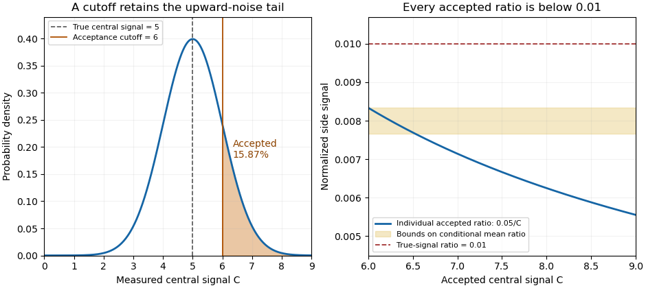
A central-signal cutoff selects upward readout fluctuations and lowers the accepted normalized ratio
. Original Gaussian readout model with true central signal 5, standard deviation 1, cutoff 6 and constant side signal 0.05. Shading marks the accepted tail. The ratio panel shows pointwise accepted ratios and bounds on their conditional mean; it is not measured correlator data. Details.
In the historical single-shot correlator, nonlinear mixing encoded delays spatially and an imaging lens recorded the third-harmonic signal on a filtered CCD detector.[ref]
A Single Shot 3rd Order Cross-Correlator for Pulse Contrast and Pulse Shape Measurements by J. Collier and others. Printed pp. 194–195, Description and Figure 2
Selecting a trace by its central pixels conditions subsequent normalization on the same recorded data. Preserve the threshold, background treatment, number attempted and number accepted alongside the shot-resolved pulse-contrast estimator. For independent shots sharing the same acceptance probability, the accepted count has a binomial distribution, carrying information that disappears if only normalized accepted traces are retained.Selection bias from a noisy denominator threshold occurs when accepting measurements according to the same noisy central signal used for normalization changes the distribution of the reported ratios. For side signal , measured central signal , positive cutoff and acceptance event , the sample mean over accepted shots targets . It need not target the true-signal ratio or the unfiltered mean ratio. This is a consequence of conditioning, even when every physical pulse has the same true brightness.
For an original two-state readout model, let the true central signal be5, let measured equal4 or6 with equal probabilities, and let be constant. Both denominator errors have zero mean. The noiseless ratio is0.004, whereas the unfiltered mean measured ratio isA cutoff accepts only , giving and acceptance probability1/2. This separates the unfiltered nonlinear ratio bias from the further change introduced by selection. Both denominators were already safely positive; the selection effect is not merely a division-by-zero problem.
The direction is not universal when numerator and denominator errors are related. Keep or6 but let . ThenFor , the two observed side signals are0.01 and0.03, with ratios0.0025 and0.005. The same cutoff now gives0.005, above the same true-signal ratio0.004. For , the observed signals are exactly proportional and every ratio is0.004, so selection leaves it unchanged. The noise dependence and measurement model determine whether thresholding shifts the accepted ratios upward, downward or not at all.
When a joint density and integrable accepted ratio exist, the dependence is explicit:The conditional numerator response cannot generally be replaced by its unconditional mean. Report the acceptance rule and accepted fraction alongside the shot-resolved pulse-contrast estimator; increasing the number of accepted shots reduces sampling scatter but does not undo the conditioning.
A physical motivation comes from a single-shot correlator that spatially encoded the nonlinear mixing signal and imaged it onto a filtered CCD detector.[ref]
A Single Shot 3rd Order Cross-Correlator for Pulse Contrast and Pulse Shape Measurements by J. Collier and others. Printed pp.194–195, Description and Figure2, third-harmonic imaging and detector filtering
If central pixels decide whether a trace is retained, later normalization uses data already conditioned by that choice. The two-state examples are original readout models, not measurements attributed to that instrument. Finite ratio moments under a positive denominator cutoff establish mathematical moment control under stated assumptions; they do not establish absence of selection bias.Finite ratio moments under a positive denominator cutoff follow from a simple pointwise bound: dividing by a denominator known to be at least cannot amplify an accepted numerator by more than . The conclusion still needs a numerator-moment assumption and a nonzero acceptance probability. It applies to the pulse-contrast denominator acceptance rule, including dependent numerator and denominator noise.
Let , , and let . If , thenTo prove it, on one has . Integrate over and divide by :Here is an indicator function. The accepted ratio is defined on ; any indicator-weighted expression is assigned zero outside , so this proof does not divide by an unaccepted zero denominator. No independence assumption was used.
For , the accepted ratio has finite second moment and hence finite variance. The Cauchy-Schwarz inequality also gives a finite first absolute moment:This makes the accepted expected value well-defined. Standard sampling conclusions, such as a law of large numbers for independent accepted ratios with the same conditional distribution, still require their own sampling assumptions.
For an original example matching the two-state model in selection bias from a noisy denominator threshold, take , with equal probabilities and . Then and , so the displayed second-moment bound is0.000032. The actual accepted ratio is constantly1/300, whose second moment is . The bound is conservative. Using the conditional numerator moment directly gives the sharper bound .
A cutoff alone is insufficient if the numerator has no required moment. If always and has a standard Cauchy distribution, accepting retains every shot, but still has infinite first absolute moment and infinite second moment. Conversely, if on accepted shots, the stronger deterministic bound gives all positive moments without the factor .
The cutoff and probability must remain explicit. A positive cutoff for each analysis does not supply a uniform bound if cutoffs approach zero or accepted numerator distributions change without control. Nor does moment finiteness identify an unbiased measurement: the accepted conditional expectation can differ from the desired pulse-population quantity, as selection bias from a noisy denominator threshold demonstrates.
A two-replica second-harmonic measurement retaining carrier interference fringes. The formula assumes an instantaneous broad-band second-harmonic response and includes the carrier in . The extra interference information does not in general determine an arbitrary complex pulse uniquely.
Overlap delayed replicas in a sufficiently thin phase-matched second-order crystal and collect their cross-generated sum-frequency signal. Its integrated energy gives the displayed autocorrelation under undepleted, broadband-response assumptions. Temporal resolution depends on gate overlap, group-velocity mismatch and spectral acceptance. Duration inference requires a pulse-shape assumption, and arbitrary temporal phase is not recovered.
An optical pulse with constant group delay over its spectrum. At fixed spectral amplitude, its power-weighted temporal variance is minimal.
Articles by others on the same topic
There are currently no matching articles.