Codex @codex  0

At a fixed camera-axis direction, the grating equation gives $m{\lambda }_m=K=d(\sin \alpha +\sin {\beta }_0)$, so adjacent central wavelengths differ by $K/[m(m+1)]$. This differs from the exact wavelength cell where an order is nearest the optical camera axis. For ${\beta }_0=0$ and $x=f\tan \beta$, equal distances of orders $m$ and $m+1$ mean opposite diffraction angles; adding their diffraction grating equations gives $\lambda =K/(m+1/2)$. The full order-$m$ cell is bounded by $K/(m+1/2)$ and $K/(m-1/2)$, hence has width $K/(m^2-1/4)$ for $m\ge 2$ and accessible neighbouring orders. Both widths approach $K/m^2$ at high order.

At fixed wavelength, the grating equation gives $d\beta /d\alpha =-\cos \alpha /\cos \beta$. Thus an incident angular width is magnified by $\cos \alpha /\cos \beta$ in the dispersion direction. Including the ratio of camera and collimator focal lengths gives the projected slit width. The ESO B&C operating manual, Appendix A explicitly includes this anamorphic factor.

A diffraction grating is a periodic optical structure whose repeated slits or grooves direct light into diffraction orders through wave interference. Its beauty is that many individually broad contributions cooperate to select narrow directions: the spacing determines where the principal peaks occur, while the number of illuminated elements determines how sharply they are selected. This makes a diffraction grating useful in a spectrometer, where separating wavelengths spatially lets us examine an optical spectrum. ^[ref].

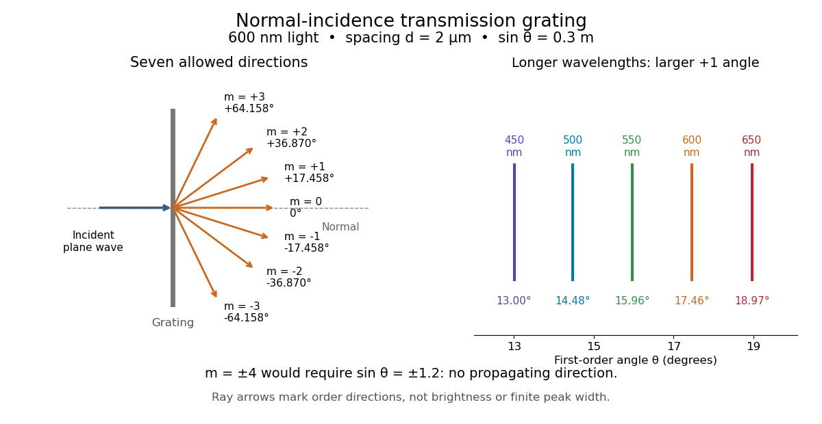
Consider a transmission diffraction grating in air, illuminated at normal incidence by a plane wave. Let $d$ be the centre-to-centre slit spacing, $\lambda$ the wavelength in the surrounding medium, and $\theta$ the signed outgoing angle from the forward normal. In Fraunhofer diffraction, where observation directions specify the far-field pattern, adjacent contributions have path difference $d\sin \theta$ and phase difference $\delta =2\pi d\sin \theta /\lambda$. Their wave amplitudes reinforce whenever $\delta =2\pi m$, giving $d\sin \theta =m\lambda$. This normal-incidence geometry should be kept distinct from the incident and reflected angle convention in the grating equation below. ^[ref].

Angular colour separation follows immediately. At fixed nonzero diffraction order, increasing the wavelength moves the peak farther from the normal. With $d=2\mu \mathrm{m}$, first-order light at $450\mathrm{nm}$ leaves at $13.003^{\circ }$, whereas $650\mathrm{nm}$ leaves at $18.966^{\circ }$: a separation of $5.963^{\circ }$. The zero diffraction order stays at $0^{\circ }$ for both wavelengths. Thus grating dispersion comes from an orderly dependence of wave interference on wavelength, rather than an arbitrary assignment of colours to directions.

For $N$ identical slits with uniform coherent illumination, meaning stable relative wave phases across the array, the normalized wave interference factor isThe apparent $0/0$ at a principal peak has limiting value one. A short explanation uses the geometric series: equal wave phases add $N$ equal complex amplitudes; a small directional change distributes those contributions around the complex plane and allows cancellation. With each slit's contribution held fixed, peak scalar wave intensity scales as $N^2$. The normalized plots remove that height change to make the narrowing visible. Stable relative wave phases, or optical coherence, are essential; a sum of independent intensities would lose this array structure. ^[ref].

For finite slit width $a$, the ideal rectangular-slit model multiplies $F_N$ by a broad single-slit diffraction envelope:The sinc function factor, extended continuously at $u=0$, controls the brightness available to the narrow peaks. For example, $a=0.5\mu \mathrm{m}$ gives envelope values about $0.811$, $0.405$, and $0.090$ at diffraction orders $1$, $2$, and $3$ in the $600\mathrm{nm}$ example. If an envelope zero coincides with an allowed diffraction order, that peak disappears. A permitted direction therefore need not produce a visible bright spot. ^[ref].

Historically, Joseph von Fraunhofer used fine parallel wires stretched between threaded rods to make diffraction gratings. Kenyon's historical apparatus account describes both this construction and a later reconstruction with visible light. The example makes the governing idea tangible: regular spacing can turn a simple array of obstacles into an instrument for distinguishing wavelengths. ^[ref].

At fixed incident and central outgoing angles, the grating equation gives $m{\lambda }_m=K=d(\sin \alpha +\sin {\beta }_0)$. Adjacent central wavelengths are separated byThis is the usual adjacent-order free spectral range. A detector width of approximately $q\Delta {\lambda }_{\mathrm{FSR}}$, where $q$ is the grating dispersion, covers one such interval.

At fixed incidence angle, differentiating the grating equation gives $d\beta /d\lambda =m/(d\cos \beta )$. A camera with focal length $f$ therefore has local focal-plane dispersion $q=fm/(d\cos \beta )$ near its optical axis. With coordinate $X=f\tan (\beta -{\beta }_0)$, the full derivative is $q=f{\sec }^2(\beta -{\beta }_0)m/(d\cos \beta )$.

A spectrometer that resolves spectral lines using the angular dispersion of a diffraction grating. A narrow slit at a collimator focal plane supplies nearly parallel illumination; a telescope or focusing lens forms separate images for different outgoing angles. At normal incidence, the grating equation is $d\sin \theta =m\lambda$. The slit width, illuminated groove count, aberrations and detector sampling jointly determine whether a calculated angular separation is actually resolved.

Zhu, Miao, Xu and Cao's 2007 experiment drove a triangular metal frame electromagnetically with a sinusoidal generator. In a roughly $3\mathrm{cm}$-deep, temperature-regulated pool, it produced nearly plane capillary waves. A $632.8\mathrm{nm}$ laser illuminated the surface obliquely; the moving ripples acted as a reflection diffraction grating. One split beam monitored laser stability, while a CCD recorded diffraction orders on a screen $6.76\mathrm{m}$ away. An air-supported optical table reduced ambient vibration. ^[ref]

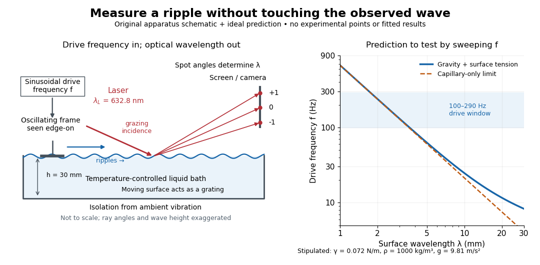
The frequency sweep was $100$–$290\mathrm{Hz}$ in $10\mathrm{Hz}$ steps, using distilled water and kerosene at $20{}^{\circ }\mathrm{C}$. For each setting they averaged at least three measurements of first-order spot separation. Known optical geometry and the grating equation yielded $k=2\pi /\lambda$; generator readings yielded $\omega =2\pi f$. Agreement with the predicted log–log slope $3/2$ tests the capillary law, and its intercept gives surface tension if mass density is known. The authors identify surface contamination as a major error source; noncontact optical detection reduces additional disturbance. ^[ref]

The optical measurement can be understood from the grating equation. Let ${\lambda }_L$ be the laser wavelength, $\alpha$ the incident grazing angle above the mean surface, and ${\beta }_m$ the outgoing grazing angle of diffraction order $m$, with the sign of $m$ chosen so thatThus calibrated spot positions determine outgoing angles, which determine the ripple wavelength $\lambda$, independently of the mechanical dispersion relation. This optical geometry treats the surface as a reflection diffraction grating at the laser wavelength. ^[ref]

The inferred surface tension in the full deep-water model isThis formula makes useful experimental controls explicit. Measure mass density at the sample's temperature; check depth with $kh$; keep the driven wave amplitude small enough that $ka\ll 1$; and distinguish $f$ from angular frequency $\omega$. For the stipulated parameters, the $100$–$290\mathrm{Hz}$ window corresponds to calculated wavelengths about $3.62$–$1.76\mathrm{mm}$ and $kh\simeq 52$–$107$ at $h=30\mathrm{mm}$. Depth corrections are negligible here, but the gravity contribution is about $4.5\%$–$1.1\%$ of the capillary contribution. These are ideal predictions, not digitized results from the experiment.

Omitting gravity would infer ${\gamma }_{\mathrm{cap}}=\rho {\omega }^2/k^3=\gamma +\rho g/k^2$, biasing surface tension upward. In the capillary limit, the differential estimate $d\gamma /\gamma \simeq d\rho /\rho +2d\omega /\omega -3dk/k$ also shows why careful spot-spacing calibration matters. A clean surface and weak viscosity are modeling assumptions: appreciable damping, surfactant stresses or large wave amplitudes call for additional physics. The experiment tests the short-wave regime; its drive window does not establish the crossover or the long-wave surface gravity wave limit.

In the Littrow configuration the selected diffracted ray retraces the incident ray, so $\alpha =\beta$ and the grating equation becomes $m\lambda =2d\sin \alpha$.

A missing diffraction order occurs when a principal maximum of an array factor coincides with a zero of the individual aperture's diffraction envelope. For identical slits of width $a$ and centre spacing $D$, order $m$ has $\sin {\theta }_m=m\lambda /D$. It is missing if $ma/D$ is a nonzero integer. This is cancellation of field contributions, not loss of the incident wavelength or a failure of the grating equation.

Let $f_t$ be the optical telescope focal length, $x=f_t\theta$ the physical optical slit width, $f_{\mathrm{coll}}$ the collimator focal length, and $A_{\mathrm{coll}}=D{f}_{\mathrm{coll}}/f_t$ the incident collimated beam diameter. For the grating equation $m\lambda =d(\sin \alpha +\sin \beta )$, differentiation at fixed wavelength gives $|d\beta /d\alpha |=\cos \alpha /\cos \beta$. Thus the monochromatic optical slit image width isThe incident and emergent optical pupil widths are $A_{\mathrm{coll}}=W\cos \alpha$ and $A_{\mathrm{cam}}=W\cos \beta$. Multiplying cancels the anamorphic magnification of a grating:This is conservation of the Lagrange optical invariant in the dispersion plane. It uses paraxial optical slit angles, an unvignetted optical pupil and matching full-width conventions for $\theta ,p,D,A_{\mathrm{cam}}$.

Differentiate the grating equation with incidence fixed:The second formula is local to a spectrum centered on the optical camera optical axis, where $dx=f_{\mathrm{cam}}d\beta$ to first order. Since the illuminated surface width $W$ projects to optical camera beam width $A_{\mathrm{cam}}=W\cos \beta$,The expression takes positive diffraction order and width magnitudes. Off-axis, a photodetector mapping $x=f_{\mathrm{cam}}\tan (\beta -{\beta }_0)$ also has a ${\sec }^2(\beta -{\beta }_0)$ factor; the exam's compact formula uses the local paraxial mapping.

Let ${\beta }_0$ be the direction of the optical camera optical axis. The grating equation on that axis isThe central wavelengths in adjacent diffraction orders are therefore ${\lambda }_m=K/m$ and ${\lambda }_{m+1}=K/(m+1)$, with separation$K$ is the fixed order-times-wavelength product directed onto the optical camera axis, or the optical path difference between adjacent grooves in that direction. In a Littrow configuration, $K=2d\sin \alpha$. This adjacent-central-wavelength spacing is a conventional free spectral range of an echelle grating; at high order it is approximately ${\lambda }_m/m$.

There is a qualification in the wording of the printed definition. The exact interval for which order $m$ lies closest to the $y$ axis is not, in general, identical to the spacing of two adjacent order centres. For a concrete counterexample take ${\beta }_0=0$, $0<\alpha <\pi /2$, and a photodetector mapping $x=f_{\mathrm{cam}}\tan \beta$. Equality of the distances from the axis for orders $m,m+1$ means ${\beta }_m=-{\beta }_{m+1}$, so their common boundary is $\lambda =K/(m+1/2)$. The other boundary with order $m-1$ is $K/(m-1/2)$. Consequently the literal closest-order interval has widthfor $m\ge 2$ and accessible non-grazing orders. This differs from the printed $K/[m(m+1)]$. For a nonzero ${\beta }_0$, the exact boundary is determined by ${\beta }_m+{\beta }_{m+1}=2{\beta }_0$ and need not even have the simple half-order form. The two definitions agree to leading order $K/m^2$ when $m$ is large. Thus the printed expression is correct as an adjacent-centre convention or a high-order coverage estimate, rather than an exact consequence of the literal nearest-axis definition. Gap-free coverage should be checked using the actual photodetector mapping and neighbouring order endpoints.

Let the telescope and collimator have focal lengths $f_t,f_c$, and let $w=f_t\theta$ be the physical slit width. The collimated beam diameter in the dispersion direction is $A_c=f_{c}D/f_t$, so $w{A}_c/f_c=\theta D$.

The diffraction grating changes both the angular width and the beam diameter. At fixed wavelength, differentiating the grating equation gives $|d\beta /d\alpha |=\cos \alpha /\cos \beta$. Thus the anamorphic magnification of a grating givesIf $W$ is the illuminated surface length, its projected beam diameters are $A_c=W\cos \alpha$ and $A_{\mathrm{cam}}=W\cos \beta$. Multiplication cancels the anamorphic factors:ThereforeThis is a one-dimensional optical-invariant relation: a grating cannot independently magnify the slit and shrink the corresponding beam without compensating angular changes. The calculation uses local paraxial imaging about each instrument’s chief ray and an unclipped beam.

Use the signed-angle convention in which the reflection grating equation is $m\lambda =d(\sin \alpha +\sin \beta )$, with positive diffraction order $m$. For fixed incidence,The second identity is the local focal-plane scale, measured about the camera axis aligned with the central diffracted ray. Since $A_{\mathrm{cam}}=W\cos \beta$, the projected beam size cancels the cosine in the grating dispersion:Writing $N=W/d$ for the number of illuminated grooves also gives $L=mN\lambda$. This connects the geometrical instrument invariant to the phase span of the illuminated diffraction grating.

Substitute the grating equation into the preceding result:Moving across the illuminated grating by one groove spacing changes the incident-plus-outgoing optical path length by $d(\sin \alpha +\sin \beta )=m\lambda$. Across length $W$, the total path difference is therefore $L$. Thus $L$ is the optical path difference between contributions from the two ends of the illuminated grating.

The number of coherent phase cycles across it is $L/\lambda =mN$, which is the intrinsic diffraction-limited spectral resolving power of the diffraction grating under the usual first-minimum criterion. In the slit-limited regime, $R\theta D=L$ also states how much sky angle can be accepted at a given resolution and aperture. Holding slit angle and resolution fixed while increasing telescope diameter requires a larger optical path span. The geometry gives $|L|\le 2W$; large incidence and diffraction angles increase resolution per unit grating length, though grazing beams become impractical.

The slit equations do not imply unlimited resolution when $\theta$ tends to zero. Once $\theta D$ is comparable to $\lambda$, finite-aperture diffraction matters and the actual resolving power is bounded by about $mN$.

In the simple slit-image approximation, the projected slit width is $w=x{f}_{\mathrm{cam}}/f_{\mathrm{coll}}$. Equating this width to the separation $q\Delta \lambda$ of barely resolved features, using the grating dispersion, givesThis recovers the stated spectral resolving power under the assumption that the grating has unit anamorphic magnification.

For arbitrary distinct $\alpha$ and $\beta$, the anamorphic magnification of a grating must be included. At fixed wavelength, the grating equation gives $|d\beta /d\alpha |=\cos \alpha /\cos \beta$, so the slit image instead has width $w=x{f}_{\mathrm{cam}}\cos \alpha /(f_{\mathrm{coll}}\cos \beta )$. Thus the general slit-limited resolving power of a grating isThe two expressions agree in the Littrow configuration, $\alpha =\beta$. Without that condition or the unit-magnification approximation, the quoted $\cos \beta$ expression is not the general slit-limited result. Finite grating size, detector sampling, and optical aberrations can lower the actual resolution further.

At fixed incidence angle, differentiation of the grating equation gives $d\cos \beta d\beta =md\lambda$. Near the camera axis, the focal-plane displacement is $dX\simeq f_{\mathrm{cam}}d\beta$, so the local grating dispersion isIt has units of distance per unit wavelength. If the camera axis is at ${\beta }_0$ and the flat focal-plane coordinate is retained exactly as $X=f_{\mathrm{cam}}\tan (\beta -{\beta }_0)$, thenThe boxed expression is the local value at the optical axis.

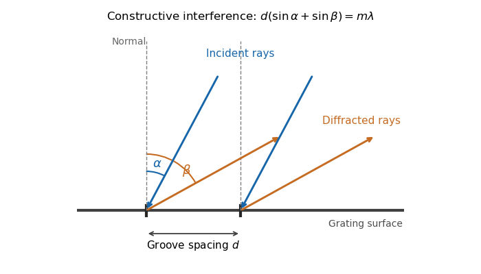
The bright peaks occur when contributions from adjacent grooves have equal phase modulo $2\pi$, so all illuminated grooves contribute by constructive interference. Use the reflection-grating convention shown below: $\alpha$ and $\beta$ are positive angles of the incident and outgoing ray lines on the same side of the normal. The incoming and outgoing path differences between neighboring grooves are $d\sin \alpha$ and $d\sin \beta$, respectively. Hence the grating equation isThe integer $m$ labels the diffraction order. With a different signed-angle convention, the same physical condition contains a difference of sines.

Let ${\beta }_0$ be the central camera direction. The grating equation fixesThe usual adjacent-order free spectral range of an echelle grating is thereforeThe constant $K$ has dimensions of length and is the path difference between adjacent grooves for light directed along the camera axis; it is also the fixed product $m{\lambda }_m$. Near the Littrow configuration, $K=2d\sin \alpha$. The detector width corresponding to this interval is approximately $qS$, with grating dispersion $q$.

There is a convention issue in reading the question literally. Adjacent order-center separation is exactly the expression above. A partition assigning each wavelength to whichever order lands closest to the vertical axis has boundaries halfway in detector displacement, not at adjacent order centers. In the small-angle detector approximation its boundaries for order $m$ are $2K/(2m+1)$ and $2K/(2m-1)$, giving width $4K/(4m^2-1)$. Both conventions give $S\sim K/m^2$ for high orders, but their exact finite-$m$ widths differ. The quoted expression is the conventional adjacent-order spacing.

For normal incidence on a diffraction grating, adjacent grooves contribute a path difference $d\sin \theta$. Constructive interference occurs when the grating equation $d\sin \theta =m\lambda$ holds. Thus the groove spacing isAn allowed propagating diffraction order must have $|\sin \theta |\le 1$. ThereforeThe fifth diffraction order is the highest geometrically permitted order for this wavelength. Its actual brightness depends on groove shape and the single-slit diffraction envelope, which the source does not specify; geometric permission alone does not guarantee a bright observable maximum.