Huber loss (${\rho }_k(u)$)

The Huber loss is quadratic near zero and linear beyond a fixed cutoff; its derivative is the clipped Huber score.

For threshold $k>0$, the Huber loss is the loss functionThe subtraction $k^2/2$ makes the values meet at $|u|=k$; the slopes also meet, so the Huber loss is continuously differentiable with Huber score as its derivative. It is a convex function, since that derivative is a monotone function. These quadratic and linear pieces define the original clipped location criterion.^[ref]

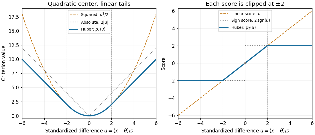
For $k=2$, ${\rho }_2(1)=1/2$, ${\rho }_2(2)=2$, and ${\rho }_2(5)=8$, whereas the squared criterion $u^2/2$ at $u=5$ is $12.5$. Increasing a standardized difference from $5$ to $6$ raises the Huber loss by $2$, but raises the squared criterion by $5.5$. The compromise preserves quadratic sensitivity to small differences while limiting the slope for large ones. This makes the Huber loss useful when ordinary observations should retain their detailed distances yet isolated outliers should exert limited pull.

For a fixed finite dataset and scale, taking $k$ large enough that every difference from the sample mean lies within $ks$ recovers that sample mean. Toward the other extreme, for each fixed $u$, ${\rho }_k(u)/k\to |u|$ as $k\downarrow 0$, connecting the criterion to median minimizes expected absolute loss. The normalization is essential: putting $k=0$ into the unscaled Huber loss gives zero everywhere, not a usable median criterion.

A Huber loss applied to a discrete gradient combines quadratic penalization of small slopes with linear penalization of large slopes. This interpolates between squared-gradient smoothing and total variation denoising, allowing smooth regions while retaining an edge-preserving large-gradient regime. The threshold should be chosen consistently with the signal's units and discretization. It can reduce staircasing in total variation denoising without guaranteeing its elimination.