
Shot noise photocurrent measurement 2026-10-18
MIT's guide uses an illuminated vacuum photodiode, with collecting anode positive relative to the emitting cathode. A transimpedance amplifier gives ; a multimeter reads its mean. The fluctuation path rejects below , adds roughly tenfold voltage gain, then nominal hundredfold preamplification and a – band-pass filter; the readout measures root mean square voltage. With diode bias off, a sinusoid at the test port calibrates . Restore bias, retain gain settings, vary lamp brightness, and repeat both readings. The guide warns about overload; it supplies a procedure, not measured results.[ref]
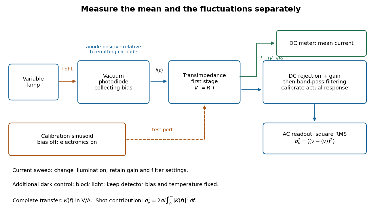
Functional photocurrent measurement: separate mean-current, fluctuation and calibration paths
. Original functional diagram organizing the laboratory's measurement roles; it is not a component-level circuit reproduction. includes current-to-voltage conversion and the complete fluctuation path. The dark comparison below is an additional control. Details.
The inference can be expressed without relying on nominal passband edges. Let denote the calibrated voltage transfer after the conversion, so and define . Under independent arrivals and an unchanged additive background,The slope of voltage variance against mean electric current can therefore estimate . A free intercept accounts for a constant background; forcing the line through zero generally biases the slope. The root mean square readings must have their mean removed and then be squared. Subtracting two root mean square amplitudes does not subtract independent variances. Estimate the variance from successive records; averaging the waveforms first would suppress the fluctuation being measured.
Additional controls sharpen this interpretation. Block the light with detector bias, temperature, and gain unchanged; this preserves dark current and electronics while removing photocurrent. Repeat this dark comparison between illumination settings to check drift. If independent dark arrivals have mean magnitude and illuminated arrivals add , their spectra add: . Subtracting the unchanged dark variance isolates . This subtraction model assumes unchanged transfers and independence; switching off bias for gain calibration is a different control and need not preserve the dark background.
Vary measured rather than assuming lamp knob position is proportional to photocurrent. Check collection versus bias to identify a range where incomplete collection is negligible; a space charge limited tube can correlate transfers. Verify that the transimpedance amplifier remains linear and that its frequency response is unchanged over the illumination range. Changing signal bandwidth should change the excess variance through ; compare inferred input spectra in several bands. Correlated fluctuations of the light source can add a contribution scaling approximately as , while an electronics floor can hide the linear term at small electric currents. A fitted line over a short range alone does not establish independent transfers.
The gain calibration must include the same detector-to-readout path used for noise, or explicitly supply any omitted transfer. Detector capacitance, finite collection time, amplifier voltage and current noise, thermal electrical noise, pickup, clipping, and finite recording precision limit the inference. Current-dependent electrical impedance or heating can make a background current-dependent too. Since contains squared gain, a small fractional error in gain produces approximately twice that fractional error in the predicted variance scale. Knowing a nominal gain and two cutoff settings is insufficient.
Thermal noise measurement 2026-10-18
MIT's laboratory guide mounts resistors on an aluminum box beneath a metal beaker shield, with short twisted leads. Its SR560 amplifier uses nominal gain before a Krohn-Hite – band-pass filter; an oscilloscope reads root mean square voltage. Calibration sweeps an attenuated sinusoid and measures the actual gain . Students alternate the resistor and a short circuit, subtracting squared readings , and disconnect the ohmmeter during noise acquisition. Lead and input capacitance enter the gain-squared integral. With settings unchanged, varying electrical resistance or temperature tests the predicted mean square. The guide prescribes repeated readings and warns against averaging noise waveforms to zero. This is a documented teaching protocol, not a supplied dataset of measured outcomes.[ref]
Johnson Noise and Shot Noise: The Determination of the Boltzmann Constant, Absolute Zero Temperature and the Charge of the Electron by MIT Department of Physics. MIT Department of Physics, Johnson Noise and Shot Noise, pp. 5–9: equation (13), apparatus §III, calibration §IV.1, Figure 5, and shorted-input subtraction equation (20)
The subtraction requires care: shorting the input changes the source electrical impedance. An amplifier's input current noise can therefore produce different voltage noise in the two configurations; a shorted baseline alone does not remove that contribution. Gain drift, interference and insufficient observation time also limit the inference. These are limitations of interpreting the measurement, not corrections that can be inferred from the nominal signal bandwidth alone. In an independent analysis one would compare the measured difference withwhere represents the measured shunt capacitance and excludes that separately modeled shunt. If calibration already includes the same shunt response, applying the denominator again counts the attenuation twice. The thermal noise worked example and both original figures illustrate ideal models; they claim no measured agreement or measured value of the Boltzmann constant.