An electric current measures how quickly signed electric charge crosses a chosen fixed oriented surface . Choose its unit normal ; positive electric charge crossing along counts positively, while crossing against it counts negatively. If is the accumulated signed electric charge transported through , thenHere is the current density; the surface integral collects its local normal contributions. Reversing the unit normal reverses . The electric current is a signed scalar associated with the whole chosen oriented surface, whereas current density is a vector at each point. The SI unit is the ampere, one coulomb per second. [ref]
https://openstax.org/books/university-physics-volume-2/pages/9-1-electrical-current. Ling, Sanny and Moebs, University Physics II, §9.1: transported charge and current
; [ref]https://openstax.org/books/university-physics-volume-2/pages/9-2-model-of-conduction-in-metals. Ling, Sanny and Moebs, §9.2: current density and its surface integral
.For a constant electric current of over a time interval of , the transported electric charge is . This need not be electric charge accumulating in the wire: in steady transport, electric charge enters and leaves. For a closed oriented surface with outward unit normal, electric charge conservation instead gives . Keeping transported and enclosed electric charge distinct connects electrical circuit bookkeeping to the local continuity equation.
A free current is the part of the macroscopic electric current assigned to mobile or externally supplied electric charges, rather than to the bound motion represented by polarization and magnetization. In a conductor, drifting conduction electrons provide a familiar example.
In macroscopic Maxwell's equations, the free-current density appears as . Here is the magnetic field strength and the electric displacement field. The separation depends on the material model; the total microscopic charge motion remains the source of the electromagnetic field.
Historical terminology for electrical effects supplied by electrochemical cells. The source supplies energy through chemical changes; the resulting electric charge and electric current obey the same electrical laws as charge supplied by other means.
A conduction current is transport of electric charge by mobile carriers through matter. For a local isotropic ohmic medium, its current density is , with electrical conductivity . It differs from displacement current , which can be nonzero in a capacitor's insulating gap without carriers crossing the gap.
An electric current that reverses direction periodically. A sinusoidal alternating current has the displayed form, where is its peak amplitude, its angular frequency, and its phase.
AC power describes energy transfer associated with time-varying electric potential difference and electric current, including the distinction between instantaneous transfer and its average. With the passive sign convention, current enters the terminal marked positive, and instantaneous power absorbed by the element is . A positive value means energy entering the element; a negative value means energy returning through that terminal pair.
For sinusoidal steady operation, choosewhere and are root mean square magnitudes. The cosine-product identity givesAveraging over a complete period removes the second term, giving active power . This derivation separates the energy-transfer average from a twice-frequency oscillation.[ref]
University Physics Volume 2 by Samuel J. Ling and others. §15.4, equations15.12–15.13, sinusoidal average power and RMS quantities
For an original example, , and give active power480W. The oscillating term has amplitude600W, so instantaneous power ranges from−120 to1080W. Over ten complete cycles at50Hz, the net energy absorbed is . Temporary negative power can accompany positive net transfer when an element stores and returns energy.
The product in volt-amperes is the apparent power. In the single-frequency sinusoidal convention, reactive power is , giving360 in reactive volt-amperes for a lagging current with . Complex electrical power packages and , while the power factor distinguishes net transfer from the terminal magnitude product. The primary MIT treatment derives these quantities and makes the peak-versus-RMS convention explicit.[ref]
AC Power Flow in Linear Networks by James L. Kirtley Jr.. Energy and Power, equations61–63; §7.1 RMS Amplitude
A measurement must retain the relative phase of the two channels. Multiplying separately measured RMS magnitudes gives apparent power, not generally active power. For nonsinusoidal signals, the time average of remains the definition of active power, but one phase angle need not describe every harmonic contribution.
The harmonic active power sum expresses average electrical power as the sum of contributions from matching components of periodic terminal electric potential difference and electric current. With a common fundamental frequency and root mean square magnitudes for nonzero harmonic components, writeHere are the signed DC components. The passive sign convention makes the average product absorbed active power. Averaging over a complete fundamental period givesFor finite sums this follows from the cosine-product identity: products of different integer harmonic components average to zero, and matching components give half the cosine of their relative phase. For square-integrable periodic waveforms, the corresponding Fourier series identity follows by continuity of the inner product in the mean-square norm. The orthogonality is a property of the averaging interval and basis, not an assumption that the physical sources are independent.
For an original example, set , , , , and fundamental relative phase . Add third-harmonic magnitudes , with relative phase . ThenThe third-harmonic contribution is , even though the total absorbed active power is positive. The root mean square values satisfy and , so apparent power is about and total power factor about .
For a purely sinusoidal supply with no DC component, only survives, giving even if the electric current is distorted. Current in other harmonic components can still increase conductor heating. The usual one-frequency complex electrical power construction is derived in the primary MIT treatment; the sum above applies that average-product reasoning separately to orthogonal components.[ref]
AC Power Flow in Linear Networks by James L. Kirtley Jr.. Energy and Power, equations 45–63; §7.1, RMS amplitudes
A proposed measurement records the two waveforms synchronously and compares their directly averaged product with the resolved sum. A non-integer-period window, unresolved harmonic components, channel timing error or changing waveform can spoil the simple finite-record equality. The formula assumes a shared periodic model; multiplying separately measured RMS magnitudes gives apparent power instead.
The power factor is the ratio of active power to the product of RMS terminal electric potential difference and electric current:when the denominator is positive. It measures how effectively those terminal magnitudes support net average transfer. With signed absorbed power it can be negative for net generation; for an absorbing load the usual range is zero to one. The Cauchy-Schwarz inequality applied to the time average of proves .
For one-frequency sinusoids, , so the power factor is . The phase-only quantity for the fundamental is also called displacement power factor. The primary treatments make the RMS convention explicit.[ref]
University Physics Volume 2 by Samuel J. Ling and others. §15.4, equations15.12–15.13
[ref]AC Power Flow in Linear Networks by James L. Kirtley Jr.. Energy and Power, equation62; §7.1 RMS Amplitude
A distorted current can give another result. For purely sinusoidal supply potential difference and a zero-mean current with fundamental RMS magnitude ,Only the in-phase fundamental contributes to the average product with that supply waveform. For an original example with fundamental3A in phase and third-harmonic RMS magnitude4A, total RMS current is5A. The displacement power factor is one but total power factor is0.6. Changing the fundamental phase alone would not remove this harmonic-current contribution.
At fixed absorbed active power and supply RMS potential difference, . For an original900W,230V example, changing the factor from0.6 to0.9 changes source current from about6.52 to4.35A. In the same upstream resistance, the corresponding loss becomes of its former value. This is a stipulated circuit calculation, not an assertion about a particular tariff or installation.
Power factor correction addresses the mechanism causing the low ratio. An ideal capacitive branch can offset inductive reactive power at one frequency; it does not automatically correct an arbitrary distorted current. State the waveform conditions and whether the reported number is total or displacement factor when comparing measurements.
A lagging power factor describes an absorbing sinusoidal electrical load whose electric current lags its terminal electric potential difference. With the passive sign convention, chooseThe current maximum occurs later by . The RMS phasors give complex electrical powerIn this equation the supply phasor is the real number , while denotes the conjugate of the current phasor. Positive is inductive reactive power under this convention. The primary MIT notes derive the conjugation and the peak-versus-RMS factor.[ref]
For an original , example with , active power is and reactive power is . At , radians corresponds to a current delay of about . The factor gives the magnitude of the phase relationship, while the word lagging supplies the direction lost by the cosine.
An ideal inductor is the limiting case : it alternately stores and returns magnetic energy, with zero mean active power. An absorbing resistive-inductive load usually has both positive active power and positive reactive power. An ideal parallel capacitor can reduce the source's quadrature electric current; sufficient extra capacitance eventually crosses into leading power factor rather than improving the factor indefinitely.
For distorted waveforms, specify whether lagging refers to the fundamental displacement power factor; one phase angle does not characterize arbitrary harmonic components. A signed meter display is also not a universal lead/lag label. The manufacturer's sign-convention explanation distinguishes phase direction from the convention used for displayed factor signs.[ref]
Power factor sign conventions in Schneider Electric FAQ FA212521. Resolution, lead/lag description and IEC/IEEE display-convention diagrams
A leading power factor describes an absorbing sinusoidal electrical load whose electric current leads its terminal electric potential difference. Under the passive sign convention, writeThe current maximum occurs earlier by . The complex electrical power isThe negative reactive power is consistent with a capacitive terminal response. It does not imply negative mean absorbed active power.
For an original , example with , the power factor magnitude is , active power is , and reactive power is . At the current leads by . A load with the same RMS magnitudes and the opposite phase displacement has identical active power but a lagging power factor and opposite reactive power.
For an ideal capacitor, gives a quarter-cycle current lead. Its mean active power is zero, although instantaneous power alternates as electrical energy enters and leaves the field. The primary one-frequency power derivation separates this quadrature exchange from net energy transfer.[ref]
An inductive load can acquire a leading power factor at the source when power factor correction supplies more capacitive reactive power than the load absorbs. The current reduction interval for shunt reactive compensation shows why mildly leading operation can still draw less source electric current than no correction, while excessive correction reverses that benefit.
Record phase direction or signed reactive power together with the numerical factor. The same positive cosine can describe leading and lagging loads, and a meter may assign a separate sign according to its display convention.[ref]
Power factor sign conventions in Schneider Electric FAQ FA212521. Resolution and IEC/IEEE convention diagrams
For nonsinusoidal signals, state whether leading describes the fundamental displacement power factor; the complete power factor also depends on waveform distortion.The current distortion factor is the ratio , where is the root mean square magnitude of the fundamental electric current component and is the root mean square magnitude of the complete electric current. Its square is the fraction of the current's mean square supplied by the fundamental component. This ratio is distinct from displacement power factor, which measures the relative phase of the fundamental potential difference and current.
Use a Fourier series at fundamental frequency :Here is the DC component and the are RMS magnitudes of harmonic components. Averaging over a complete period, orthogonality and the Parseval identity giveFor purely sinusoidal electric potential difference , only the fundamental electric current contributes to active power:Thus a displacement power factor of one can coexist with a lower total power factor.
For , use fundamental-normalized current total harmonic distortion, . The relation between current distortion factor and THD with DC current isWith zero DC component, this reduces to . The definition of RMS here includes the DC component. For example, a 10 ampere fundamental and 3 ampere DC component, with no higher harmonic components, have zero total harmonic distortion but .
For an original zero-mean waveform, take a 230 volt RMS sinusoidal supply, , , and RMS third/fifth harmonic components of 6 and 3 amperes. ThenThe active power is 1840 watts, apparent power is about 2769.57 volt-amperes and total power factor is about 0.6644. This is an illustrative waveform model, not a measurement of a particular rectifier.
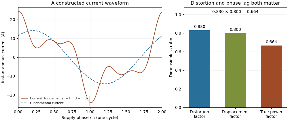
Terminology requires care. Overview of Functions: Harmonic Measurements by Schneider Electric uses distortion factor for the ratio of power factor to the fundamental cosine. Power Quality Considerations by Schneider Electric uses the label for harmonic content relative to the fundamental, or total harmonic distortion. The defining ratio identifies the intended quantity.
If the supply also contains harmonic components, use the harmonic active power sum:with matching voltage/current phase conventions. The fundamental-only factorization above assumes a purely sinusoidal supply.
The relation between current distortion factor and THD with DC current accounts for the mean component omitted from the usual fundamental-normalized total harmonic distortion. For a periodic electric current, let be its signed DC component, the fundamental RMS magnitude, and the RMS magnitudes of higher harmonic components. The Parseval identity givesDefine and current distortion factor . Division by provesThe root mean square in this expression includes the mean, while the stated total harmonic distortion excludes it. An instrument reporting AC-only RMS or a differently normalized distortion quantity requires a correspondingly different conversion.
For an original example, take , and combined higher-harmonic RMS magnitude . Then , and . Neglecting the DC component would instead predict . In the same conductor electrical resistance , the actual heating is , while that omission would predict .
For a zero-mean sinusoidal supply of RMS and an in-phase fundamental current, the example absorbs . Its apparent power is approximately , so total power factor is despite a displacement power factor of one. The DC component carries no average power from that particular zero-mean supply, but it still increases mean-square electric current. If the supply itself has a DC component, its contribution must be included through the harmonic active power sum.
As tends to zero the defining current distortion factor can tend to zero, but fundamental-normalized total harmonic distortion is undefined at . Do not evaluate the boxed relation there by silently dividing by zero. The manufacturer's documentation also uses differing labels for distortion ratios, reinforcing the need to state the defining normalization.[ref][ref]
Overview of Functions: Harmonic Measurements by Schneider Electric. Quality Indicators, Distortion Factor
Power factor correction changes the current drawn from a source so that a specified active power is supplied with a more favorable power factor. For a sinusoidal inductive load, a parallel capacitor can supply an opposite reactive power component. It changes the source current's quadrature component while an ideal lossless correction branch leaves the load's active power unchanged.
Let the original load absorb at RMS potential difference and angular frequency . A parallel ideal capacitance contributes , soTo change a lagging phase angle from to a smaller lagging angle at fixed ,These follow from complex electrical power and the capacitive phase relationship.[ref]
AC Power Flow in Linear Networks by James L. Kirtley Jr.. Energy and Power, equations61–65; capacitive/inductive terms in equation71
For an original ideal example, take , and50Hz. An initial factor0.8 corresponds to750var. A target factor0.95 corresponds to about328.68var, so a capacitance about33.53µF supplies the difference. RMS source current changes from6.25A to about5.26A. Resistive feeder loss at fixed resistance changes by , while the1000W load conversion remains the same in this model.
Reactive power overcompensation occurs if the capacitive contribution exceeds the intended inductive component. The net then changes sign; continuing to add capacitance does not keep improving the magnitude of the factor. At a different load or frequency the same component can produce another result. Component ratings and nonideal circuit behavior require their own model rather than being determined by this one-frequency algebra.
Correction of displacement power factor is also distinct from correction of waveform distortion. Harmonic current can remain after the fundamental quadrature component is canceled. A useful measurement compares synchronized source potential-difference/current waveforms, RMS magnitudes and their average product before and after a change, retaining the operating condition. Separately measuring only RMS magnitudes cannot establish the resulting active power.
Automatic power factor correction adjusts a correction device as the measured load changes, rather than leaving one fixed compensating setting connected. In a staged capacitor bank, a controller uses terminal electric potential difference and electric current information to choose which stages are connected. The controlled quantity and target must distinguish active power, signed reactive power, waveform distortion and the chosen lead/lag convention.
For an original single-phase sinusoidal model, available stages each supply of capacitive reactive power at the operating electric potential difference. With connected stages,At fixed , maximizing the magnitude of the power factor chooses the available integer minimizing . Away from the end limits, nearest-stage rounding leaves . This capacitor-stage quantization error can be positive or negative. A policy forbidding leading operation instead restricts , so it can choose a different setting.
Suppose , and . Three stages leave and factor about leading; two stages leave and factor about lagging. Both outcomes are consistent with their respective objectives. If the load changes to , , leaving all three stages connected produces ; zero stages is closer to cancellation than one. A stored stage decision must therefore be updated when the load changes.
Actual feedback must measure the corrected network. The Eaton paper places the current transformer so it senses the relevant load and capacitor contribution, and explains how a wrong phase, polarity or location produces misleading feedback.[ref]
Capacitor Application Issues by Thomas M. Blooming and Daniel J. Carnovale. Section VI.C, printed p.8, CT Location for Automatic Banks
Measuring only the correction branch would not establish the combined source power factor.A proposed controller test varies a known resistive-inductive load through several operating points, recording stage state, signed reactive power, RMS electric current and synchronized terminal waveforms. Check both increasing and decreasing demand, including small excursions around a stage threshold. A dead band and timing rules can prevent repeated switching in response to small fluctuations; they must be specified along with the target. Stage size, switching transients and the load's harmonic components require additional checks beyond the ideal rounding model.
Capacitor-stage quantization error is the residual reactive power caused by choosing among discrete settings of a capacitor bank instead of a continuously adjustable correction. In a fixed sinusoidal operating model, let the load absorb and let the target residual be . The desired capacitive correction is . Selecting available correction leavesThe error concerns the selected setting, separately from sensing error, changing load and component tolerance.
For equal stages of magnitude and an available range covering the desired correction, nearest-stage selection chooses an integer nearest . HenceAt a half-stage tie either neighbor attains the bound. A policy forbidding a negative residual relative to zero instead rounds downward and gives , away from the bank's capacity limits. The two policies solve different constrained problems.
For an original zero-target example, let and . Three stages give ; two give . With active power , nearest-stage selection guaranteesprovided the zero-reactive target is within range and the sinusoidal fixed-load assumptions hold. At only , the same worst-case bound falls to about . A stage size suitable at high demand need not give the same numerical power factor at low demand.
Unequal stages require the actual attainable set. Stages of 100 and 400 vars permit vars. At a desired 250 vars, the nearest setting leaves 150 vars error, despite the smallest stage being only 100 vars. The relevant bound is half the largest gap between neighboring attainable settings in the tested range, not half the smallest component. Outside the bank's range, clipping to an endpoint can leave a larger error.
At fixed frequency, a fixed capacitance gives , so stage magnitudes also change with RMS electric potential difference. Eaton's paper describes discrete stage sizes, combinations and automatic control; the error bounds above are original consequences of that ideal setting model.[ref]
Capacitor Application Issues by Thomas M. Blooming and Daniel J. Carnovale. Section V.C–D, printed p.6, stage sizes and fixed versus switched capacitors
A proposed test records the actual stage states and terminal quantities while slowly varying a known load across thresholds. Compare the observed residual with the attainable-setting prediction before assigning every deviation to quantization.Optimal shunt capacitance for sinusoidal power factor correction minimizes the source's RMS electric current for an ideal fixed sinusoidal supply and a fixed load with active power and inductive reactive power . A lossless parallel capacitor supplies signed reactive power , where is the supply RMS electric potential difference and the angular frequency.
The squared source electric current isDifferentiating givesThus the unique minimum isThe fundamental quadrature electric current vanishes there. Strict convexity proves this is a global optimum in the stated model, rather than merely a stationary point. The capacitive sign and one-frequency complex electrical power relation follow from the primary MIT derivation.[ref]
AC Power Flow in Linear Networks by James L. Kirtley Jr.. Energy and Power, equations 61–65 and 71; §7.1 RMS amplitudes
For an original example, , , and give . Source electric current falls from to . A capacitance 20% below or above leaves or , respectively, and both draw about . They have the same power factor magnitude, about , but opposite lead/lag direction.
The exact excess above the optimal squared electric current isSmall sizing errors therefore affect this loss objective quadratically around the optimum, while residual reactive power changes linearly and changes sign. An allowed interval clips the optimum to its nearest feasible point. If the original load has , the constrained optimum for added nonnegative capacitance is instead .
The result assumes a fixed load, ideal sinusoidal supply, lossless correction and no additional network effects. It does not optimize a system with waveform distortion, component heating, variable terminal electric potential difference or discrete stages. The current reduction interval for shunt reactive compensation describes a wider set of beneficial choices, while automatic power factor correction follows a changing load with available stages.
Reactive power overcompensation occurs when capacitive correction exceeds the inductive reactive power that it is intended to cancel. Under the passive sign convention and a positive-frequency sinusoidal supply, the source then sees negative net reactive power, producing a leading power factor. This can happen when a fixed capacitor bank remains connected as the inductive load falls. Eaton's application paper discusses excessive leading operation and the use of switched correction stages.[ref]
Capacitor Application Issues by Thomas M. Blooming and Daniel J. Carnovale. SectionV, printed p6, switched-bank control and overcompensation
Consider an ideal fixed RMS electric potential difference at angular frequency , supplying a load that absorbs constant and . Let be the magnitude of the correction's reactive power; its signed contribution is . Adding ideal shunt capacitance givesThe model holds the load and supply fixed while changing . It omits losses and additional network dynamics. Optimal shunt capacitance for sinusoidal power factor correction follows by minimizing the squared root mean square electric current:For the remaining reactive power is positive and the power factor is lagging. For it is negative and the power factor is leading. The overcompensation threshold is , but the current reduction interval for shunt reactive compensation is wider. Comparing the square of the corrected and uncorrected electric current givesThus source RMS current is reduced for , equals the uncorrected value at , and is larger for . An overcompensated operating point between and still draws less source electric current than the uncorrected load.
For an original example, keep the parent article's chosen , , and 50 hertz. The uncorrected source draws 6.25 amperes at power factor0.8. Full cancellation needs and reduces source electric current to 5 amperes. A 100 microfarad correction gives and 5.605 amperes, with a leading factor about0.8920. A 150 microfarad correction instead gives about and7.563 amperes, worse than no correction. The crossing is .
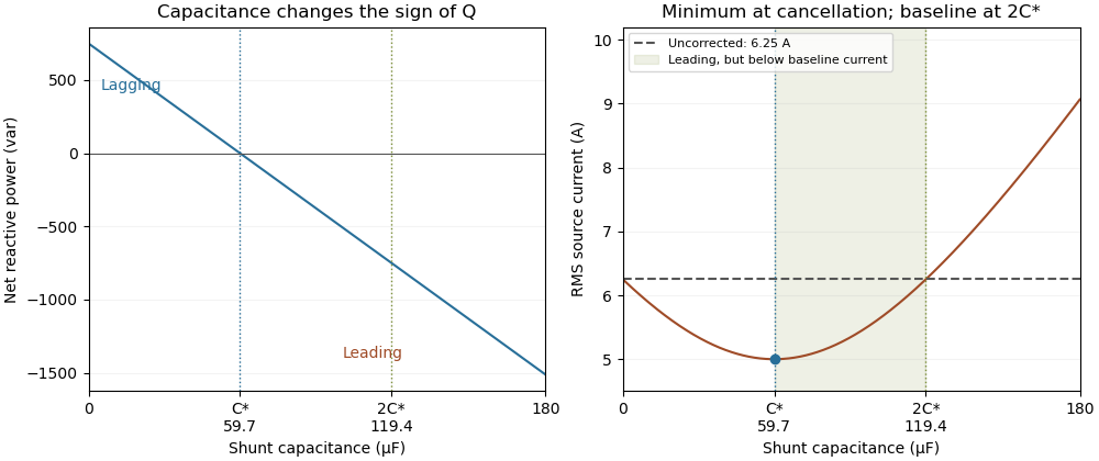
Leading operation begins before correction increases current above the uncorrected value
. Original constant-load model at 200 volts RMS and 50 hertz with 1000 watts active power and 750 vars inductive reactive power. Optimal correction is about 59.68 microfarads. Between 59.68 and 119.37 microfarads the source is leading but still draws less current than the uncorrected load; above 119.37 microfarads it draws more. Details.The optimum changes with the load. If the example load's and both halve while its original optimal correction remains connected, then and . Source electric current is 3.125 amperes and the factor is 0.8 leading. This dependence motivates automatic power factor correction. The cited controller description measures system electric potential difference and electric current, using external current transformers, and switches discrete capacitor bank stages to follow a target.[ref]
Retain the phase or sign of when reporting the result. A bare power factor magnitude does not distinguish leading from lagging; the manufacturer FAQ also illustrates how a meter's signed display depends on its convention.[ref]
Power factor sign conventions in Schneider Electric FAQ FA212521. Resolution and displayed IEC/IEEE convention diagrams
The calculation assumes sinusoidal steady state; current distortion factor is a separate consideration for nonsinusoidal current.The current reduction interval for shunt reactive compensation is the range of ideal capacitive corrections that draws less source RMS electric current than the uncorrected inductive load. It is wider than the range that avoids reactive power overcompensation.
Assume fixed sinusoidal RMS electric potential difference , active power , and inductive reactive power . Let be the magnitude of the added capacitive reactive power. Comparing squared source electric currents givesConsequentlyor with . The model's capacitive reactive power follows the sinusoidal complex electrical power convention.[ref]
At , source electric current is smallest. Between and , the source has a leading power factor but still draws less electric current than before correction. At , the residual reactive power is : its magnitude matches the original value, restoring the original source-current magnitude. Beyond that point the corrected electric current is larger.
For an original example, choose , and . Uncorrected electric current is . Full cancellation gives . An overcorrection leaves and draws only . But restores , and increases it to .
Two choices and are symmetric around the optimum and give the same squared source electric current. This symmetry explains why power factor magnitude alone cannot identify the sign of the residual reactive power. If , no positive reduces current under the same fixed-load assumptions.
With the same upstream electrical resistance, reducing source mean-square electric current also reduces that conductor's Joule heating. It does not erase the current carried by the local capacitor branch or assess its ratings. Harmonic interactions, nonideal components and changing load conditions need their own model; this interval is an exact statement about the stated one-frequency circuit.
The displacement power factor is , where is the phase difference between the fundamental components of terminal electric potential difference and electric current. It describes phase displacement at that frequency. For purely sinusoidal signals it equals total power factor; with distorted waveforms those quantities can differ. The one-frequency phase relation follows from the RMS average-power expression.[ref]
University Physics Volume 2 by Samuel J. Ling and others. §15.4, equations15.12–15.13
For a purely sinusoidal potential difference of RMS magnitude and zero-mean periodic current, orthogonality of harmonics givesThe ratio is the current distortion factor under these assumptions. A displacement factor near one does not establish that the whole current waveform closely follows the supply sinusoid.
For an original example, let the supply be100V RMS. Let the fundamental current be4A RMS at a lagging phase with cosine0.8, and add a3A RMS third harmonic. Total RMS current is5A, active power320W and apparent power500VA. The displacement factor is0.8 while total power factor is0.64.
Now cancel only the fundamental quadrature current, whose magnitude is . The remaining in-phase fundamental is3.2A and the third harmonic is still3A. RMS source current is , so total factor is about0.73 even though the displacement factor has become one. This illustrates a limitation of phase-only power factor correction, not a universal model of a correcting device.
The cosine also loses lead/lag sign: phases and have the same displacement factor but opposite sinusoidal reactive power. Retain the phase or lead/lag convention when that distinction matters. If the potential difference itself contains harmonics, total active power needs the contributions of the corresponding harmonic pairs; this simple fundamental-only reduction is no longer sufficient.
Complex electrical power represents the active and reactive parts of sinusoidal electrical energy transfer in one complex number. Using phasors and whose magnitudes are root mean square values, with the passive sign convention, defineThe star denotes a complex conjugate. The real part is active power; the imaginary part is reactive power. The magnitude is apparent power. A source using peak-amplitude phasors instead has the factor : .[ref]
AC Power Flow in Linear Networks by James L. Kirtley Jr.. Equation63 and §7.1, explicit amplitude convention
To see why the conjugate matters, write and . Then depends on the relative phase. Changing the common time reference multiplies both phasors by , leaving unchanged. The product would instead acquire and would not represent a time-reference-independent average-power quantity.
For an original example, choose and . ThenThus active power is400W, reactive power is300 reactive volt-amperes and power factor is0.8. The corresponding electrical impedance is . With RMS current magnitude5A, the resistive term absorbs , agreeing with the real part.
Under the stated sign convention and time convention, an inductive reactance gives positive and a capacitive reactance negative . Negative does not mean a negative dissipated-energy average. For example, adding an ideal parallel capacitive branch contributing cancels this example's reactive part, leaving terminal complex power400VA and RMS source current4A at100V, while the original resistive dissipation stays400W.
This one-frequency representation must not be applied indiscriminately to a distorted waveform. Different harmonics need their own phase relationships; the definition of active power remains the time average of the actual instantaneous power.
Apparent power is the product of RMS terminal electric potential difference and electric current, conventionally expressed in volt-amperes:For sinusoidal signals at one frequency, it equals the magnitude of complex electrical power and satisfies . It is not generally the average rate of net energy absorption, which is active power.[ref]
AC Power Flow in Linear Networks by James L. Kirtley Jr.. Energy and Power, equations61–63 and §7.1, apparent/complex power and RMS convention
For an original example, a100V terminal pair carrying5A RMS has500VA of apparent power. If active power is400W, the power factor is0.8. In the sinusoidal case the magnitude of reactive power is reactive volt-amperes; the magnitude calculation alone does not determine whether the current leads or lags.
Magnitudes do not add like complex quantities. Consider two parallel sinusoidal loads at the same supply, with complex powers and in volt-amperes. Each has500VA of apparent power, but the combined terminal complex power is600VA with zero imaginary part. The source therefore sees600VA rather than the1000VA sum of individual magnitudes. Their internal branch currents and individual component requirements still exist; reactive cancellation at the source does not erase those branch conditions.
For nonsinusoidal waveforms, the product definition remains useful, but the simple equality with the magnitude of one fundamental-frequency complex power needs qualification. With and , RMS current is5A and apparent power is500VA. The fundamental-frequency complex electrical power is only300VA. The extra RMS current is not represented by that one complex number.
Thus record the waveform convention with an apparent power rating or measurement. Separately measuring RMS potential difference and current gives this product, while recovering active power requires the corresponding average product or adequate phase-resolved information. The Cauchy-Schwarz inequality guarantees without assuming a sinusoidal waveform.
The volt-ampere, symbolVA, is the unit commonly used to express apparent power. At a terminal pair, RMS potential difference in volts multiplied by RMS current in amperes gives the numerical value in volt-amperes. The unit product has the same coherent SI dimensions as the watt:This unit identity does not make apparent power and active power the same quantity. The SI text explicitly warns that different physical quantities can share a unit and that the quantity must be specified.[ref]
The International System of Units (SI), ninth edition, SI Brochure. NIST SP330 parallel text, §2.3.4, coherent derived units and quantity identification
For an original example,250V RMS at8A RMS gives2000VA, or2kVA. If the absorbing load has power factor0.75, its active power is1500W. A1500W value cannot be inferred from the2kVA alone without the phase/waveform information summarized by that factor.
Hypothetical equipment can have separate apparent- and active-power limits. A1000VA/600W limit would permit a500W, factor0.5 load only at the apparent-power boundary, since it requires1000VA. A700W, factor-one load would require only700VA but exceed the separate600W limit. These examples interpret stated numerical constraints rather than specify an actual product's behavior.
For single-frequency sinusoids, the magnitude of complex electrical power is expressed in volt-amperes, while its real part is commonly expressed in watts and its imaginary part in reactive volt-amperes. Those names help keep the quantities distinct even though their base-unit dimensions agree.[ref]
AC Power Flow in Linear Networks by James L. Kirtley Jr.. Energy and Power, equations61–63; §7.1 RMS Amplitude
With distorted signals, retain the actual RMS-product definition of apparent power rather than assuming a single fundamental phasor accounts for all current.Reactive power is the imaginary part of complex electrical power in sinusoidal steady operation. With RMS phasors, the passive sign convention and time convention,where is potential-difference phase minus current phase. Inductive current lag gives positive , while capacitive current lead gives negative . Its conventional unit is the reactive volt-ampere, written var. These definitions retain the specified phasor and sign conventions.[ref]
AC Power Flow in Linear Networks by James L. Kirtley Jr.. Energy and Power, equations61–65; §7.1, RMS amplitudes
The physical role is periodic energy exchange rather than an additional dissipated-energy average. For an ideal inductor, and stored energy is , so . Its energy returns to its initial value after a steady cycle and mean absorbed power is zero. Nevertheless,For an ideal capacitor, , with the negative sign representing the opposite exchange phase. Primary circuit derivations explicitly separate these exchanges from resistor dissipation.[ref]
University Physics Volume 2 by Samuel J. Ling and others. §15.4, Figure15.16, ideal inductive/capacitive instantaneous power
For an original example, , and give . Peak stored energy is0.50J and mean stored energy0.25J, consistent with . Zero ideal average dissipation therefore does not mean zero current or zero energy storage.
For a separate ideal single-frequency compensation example, a100V load with can have its source reactive component canceled by a parallel capacitor satisfyingThe capacitor contributes , leaving400W of source active power and4A RMS source current. This illustrates power factor correction under the stated ideal assumptions, rather than selecting a real component or proving its ratings.
Reactive exchange can increase the current carried through resistive wiring and thereby affect real losses. For distorted waveforms, definitions of non-active power need additional care; the one-frequency imaginary-part definition should not silently be extended to every waveform.
The reactive volt-ampere, conventionally called the var and written with symbolvar, expresses reactive power. The official SI text notes the IEC's special name and states that its coherent unit is identical to the volt ampere. The name identifies the reactive quantity; it is not a different base-unit dimension.[ref]
The International System of Units (SI), ninth edition, SI Brochure. NIST SP330 parallel text, §2.3.4, paragraph identifying the IEC var
In sinusoidal steady operation with RMS magnitudes and relative phase ,Thus100V RMS,2A RMS and a lagging phase with give120var. Under the same passive and phasor conventions, a leading phase of equal magnitude gives−120var. The signed value describes exchange phase rather than negative dissipated heating. The prefix relation is .
A reactive-power value is also not an amount of stored energy in joules. For an ideal inductor in sinusoidal steady operation,For an original200var example at50Hz, mean stored energy is and peak stored energy is twice that. The average absorbed active power is nevertheless zero in the ideal inductor. The primary circuit treatment derives this separation between energy storage and mean dissipation.[ref]
In a sinusoidal100V example with , the reactive component is300var, the active component400W and apparent power500VA. Adding400 and300 as ordinary scalar powers would not give the500VA magnitude. Complex electrical power retains the phase relation needed for this combination.
Active power, also called real power, is the time average of instantaneous power transferred through a terminal pair. For periodic electric potential difference and electric current of common period , the passive sign convention givesThe net energy entering during each period is . Positive active power denotes net absorption under this convention; it can represent useful conversion to other forms of energy as well as heating.
For sinusoids of RMS magnitudes and with relative phase , . For a pure resistor with constant resistance , the stronger waveform-independent statement follows from :This is why the root mean square current is the constant-current value giving the same heating in that resistor.[ref]
An original harmonic example shows why RMS values alone do not determine active power. Letin volts and amperes. Orthogonality over a period gives , but the third harmonic averages to zero when multiplied by the fundamental potential difference. Consequently , whereas apparent power is . The power factor is0.6 even though the fundamental current is exactly in phase with the fundamental potential difference.
More generally, Fourier analysis of real periodic waveforms with RMS harmonic magnitudes giveswhen the expansion and average are justified. Cross terms of different harmonic orders vanish. A single fundamental-frequency complex electrical power therefore need not capture every harmonic contribution to the total average.
For an ideal inductor or capacitor in periodic steady operation, the stored energy returns to its starting value each cycle, so its net active power is zero despite nonzero exchange during the cycle. Real components can also have losses. The primary MIT treatment explicitly separates resistor dissipation from periodic inductive and capacitive energy exchange.[ref]
Electronic propagation through a device region with few momentum-randomizing scattering events. The mean free path should exceed the relevant trajectory length. Boundary specularity and aperture geometry can matter separately from the bulk mobility; electron phase coherence is an additional condition for interference.
A four-terminal bend resistance uses adjacent current contacts and the other adjacent pair as voltage probes. It can be negative when a ballistic injector preferentially populates the opposite voltage probe. Its sign is a nonlocal routing property, not the sign of the total electrical dissipation.
For a balanced nonnegative transmission matrix and , electrical power obeyswith diagonal reflection included consistently or removed from both sides. A negative four-terminal voltage-to-current ratio is compatible with this positive total power because the measured voltage pair is not the current source's pair.
For left-deflected injection in the left 1,top 2,right 3,bottom 4 geometry, use 1 to 2 with modes, 2 to 3 with , 3 to 4 with , and 4 to 1 with plus 4 to 3 with . The zero-current probes give and , hence . Reversing the transmission matrix gives equal probe potentials and zero bend resistance. Fixed-lead resistance need not be even in field; reciprocity also exchanges current and voltage pairs.
Number the leads left 1,top 2,right 3,bottom 4. Let narrow leads 1,2 have spin-resolved modes and wide leads 3,4 have . Straight-through injection sends modes between 1 and 3 and between 2 and 4; each excess mode connects 3 and 4. With current 1 to 4, and zero current at 2,3, , and . Thus . At this ideal network disconnects the current source from its drain.
A diffusion current results from a spatial carrier density gradient. For semiconductor electrons and holes in one dimension, conventional-current densities are and . Their different signs reflect negative and positive carrier charge. At equilibrium each species' diffusion current is balanced by its drift current, giving zero net current while the individual transport contributions need not vanish.
A drift current is an electric current caused by the response of mobile charge carriers to an electric field. It is distinct from the diffusion contribution due to concentration gradients. At equilibrium in a p-n junction, the two contributions cancel although each can be nonzero.
A direct current is an electric current that flows in one direction; its magnitude may vary with time. A constant or steady electric current additionally has a value independent of time. Thus a direct current need not be constant. The steady direct current model of a voltage divider assumes a constant input electric potential difference and fixed electrical resistances.
An ammeter measures electric current through a branch of an electrical circuit. Connect it in series; its own finite electrical resistance changes the measured branch's electric current unless that effect is negligible or corrected.[ref]
10.4 Electrical Measuring Instruments. Measuring Current with an Ammeter, Figure 10.35 and following paragraph: connection and loading
A galvanometer detects electric current through a mechanical response, such as the deflection of a pointer.[ref]
10.4 Electrical Measuring Instruments. Analog and Digital Meters: current-driven pointer response
A sensitive galvanometer makes a small electric current visible; a calibrated deflection also estimates its magnitude. A center-zero scale distinguishes both signs of electric current. The moving-coil galvanometer rotates a coil in an imposed magnetic field, whereas a moving-magnet galvanometer rotates a magnetic needle in the coil's magnetic field. The spring-balanced model below describes the moving-coil galvanometer, not every instrument called a galvanometer.
A current-measuring coil and compass arranged so that the coil's central magnetic field is perpendicular to the horizontal terrestrial field. With unchanged coil geometry and terrestrial field, the electric current ratio is the ratio of the tangents of the needle deflections. A small needle and controlled alignment make the central-field approximation useful.
For fixed mean turn length and fixed conductor volume, a coil of turns has conductor length proportional to and cross-sectional area proportional to . Its electrical resistance is therefore . With source electromotive force and internal resistance , suppose the small-deflection driving torque is proportional to . Its derivative has the sign of , so the maximum occurs at . Geometry, damping and finite response time can alter the practical optimization; this is a conditional winding model, not a universal rule for all galvanometers.
A galvanometer using oppositely directed, nearly equal magnetic dipole moments to reduce the net restoring torque of the approximately uniform terrestrial field. It still needs a weak restoring mechanism for a reproducible deflection; it does not shield the needles from that field.
The historical Leopoldo Nobili instrument combines a many-turn coil with an astatic needle pair. In a common geometry one needle responds strongly to the coil while its oppositely magnetized companion reduces the terrestrial restoring torque.[ref]
Astatic Galvanometer, Nobili Pattern by Museo Galileo. Inventory 1417
A small-angle galvanometer model combines its moment of inertia , damping coefficient and restoring coefficient with a torque per electric current . The resulting damped harmonic oscillator responds to the current pulse through the displayed equation. Its angular deflection can continue after the driving electric current has ceased. Inferring the current's detailed time dependence requires the instrument response, rather than equating needle angle with instantaneous current. This is a generic readout model, not a calibration of Faraday's historical instrument.
A moving-magnet galvanometer measures electric current through the torque it exerts on a movable magnetic dipole moment. A fixed coil carries the current and creates a magnetic field; a suspended magnet turns against a restoring torque supplied by its suspension or a reference field.
For sufficiently small deflections in a calibrated geometry, the coil field and resulting angular response are proportional to electric current. A pointer or reflected optical spot reads the angle. This differs from a moving-coil galvanometer, where the current-carrying coil itself moves. Mechanical damping determines whether the indication oscillates or settles smoothly after a current change.
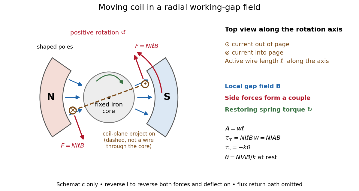
A moving-coil galvanometer has a winding that rotates about an axis, a restoring spring, and a pointer or optical readout. In the radial-field construction, a cylindrical iron core and shaped magnetic poles keep the magnetic field approximately in the coil's plane as it turns. The resulting moving-coil galvanometer torque is nearly independent of the deflection angle; the spring then converts electric current into a proportional settled deflection. [ref]
For switched on from rest, . critical damping is the fastest nonoscillatory step response at fixed natural frequency within the ordinary second-order model.
With phasors, critical damping gives , amplitude and phase . The response strongly suppresses alternating currents well above the mechanical frequency.
A galvanometer radial field is approximately radial about the rotation axis within each narrow working gap. Its direction follows the moving sides of the coil over the useful sweep. Here the magnetic field points from the left pole toward the core and from the core toward the right pole; it is not outward everywhere. This geometry keeps the magnetic force on a current-carrying wire tangential, with nearly constant lever arm. A spatially uniform magnetic field in a fixed direction would instead give an angle-dependent torque as the coil turns.
For a rectangular winding with turns, active side length , side separation , and per-turn area , the magnetic force on a current-carrying wire gives equal and opposite side forces of magnitude . Their force couple has lever arm . Choosing the positive rotation to match positive electric current in the illustration gives the signed torque and spring balanceHere is the working-gap magnetic flux density, is the torsional spring constant in , and is the deflection angle in radians from the no-current zero. The balance holds after motion has settled, within the radial-field and linear elasticity ranges. Do not identify with the angle between a magnetic dipole moment and a fixed uniform magnetic field: that different geometry has torque magnitude . [ref]
For an original illustrative design, choose , , , and . Then . At , the magnetic torque is and . Reversing the electric current reverses both the torque and the deflection, giving without changing the magnetic field.
The galvanometer current sensitivity is the change in settled deflection angle per change in electric current. In the linear model its derivative is constant, . The illustrative design has , or per . A chosen full-scale angle corresponds to ; a straight-line extrapolation beyond that range does not establish real instrument behavior.
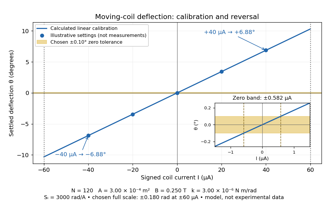
Illustrative moving-coil calibration, current reversal and finite zero resolution
. Calculated deflection for the original design, with selected calibration points and a close view of zero. The shaded band is a stipulated readout tolerance, corresponding to about ; it is not measured noise. Values and points are illustrative model predictions, not observations from a real instrument. Source. Details.Finite sensitivity and finite readable angle set different limits. Under the stipulated tolerance, a reading indistinguishable from zero means only if the zero is stable and the model applies. More turns can increase galvanometer current sensitivity while also increasing winding electrical resistance; the response to an applied electric potential difference depends on both. Friction, zero drift, departures from the radial magnetic field, and spring nonlinearity can spoil the calibration. Damping sets how long one must wait for a settled reading. A rapidly reversing electric current can produce little mean pointer deflection even when its instantaneous magnitude is large.
NCERT's teaching experiment uses a moving-coil galvanometer, a 0–6 V supply, a 0–10 kΩ series electrical resistance box , a 0–200 Ω parallel electrical resistance box , two switches and a voltmeter. With the parallel path open, close the supply switch and record the pointer deflection. Keep fixed, close the parallel path, and adjust until the deflection halves. The guide requests repeated settings, clean tight contacts and constant supply electromotive force; it introduces high before energizing to protect the winding. [ref]
Experiment 6: Resistance and figure of merit of a galvanometer. Experiment 6, printed pp. 53–58: Figure E 6.1, Procedure 1–5, Precautions and Sources of Errors
Write the winding electrical resistance as , the supply electromotive force as , and assume negligible supply internal electrical resistance. Ohm's law gives the two winding electric currentsIf proportional deflection gives , solving yields , requiring . The shortcut requires ; closing the parallel path generally changes the total supply electric current. For chosen values and , the exact result is , rather than . The manual gives this exact relation and asks how finite supply internal electrical resistance affects it. [ref]
As an additional calibration control, record the supply-off zero, apply several small positive and negative electric currents, and recheck zero after each sequence. With known, calculate each electric current from the measured supply electric potential difference and the total series electrical resistance; plot settled deflection against that electric current. Equal-magnitude reversed readings should lie equally far from a stable zero. A fitted relation separates zero offset from galvanometer current sensitivity. The manual's “figure of merit” is electric current per scale division, not the mechanical torsional spring constant used above. These reversal and zero checks extend the documented procedure; they are proposed controls, not reported measurements.
In a Wheatstone bridge, the galvanometer connects the two comparison junctions. Its purpose is to locate a null measurement, rather than to measure the branch electric current through the unknown resistor. Using Wheatstone bridge detector loading and Thévenin's theorem, a settled moving-coil galvanometer with winding electrical resistance obeysHere is the bridge's open-circuit voltage and its Thévenin resistance. For a functioning passive detector with finite positive electrical resistances, exact implies , preserving Wheatstone bridge balance. Away from balance, the detector loads the junctions; its electrical resistance cannot be ignored.
For the illustrative , and a chosen , a bridge open-circuit voltage produces and . That lies inside the stipulated zero tolerance. The corresponding resolvable open-circuit voltage scale is about , not arbitrarily small. Actual limits also depend on the zero stability and calibration.
Use the detector checks in the slide-wire resistance bridge experiment: perturb the comparison to either side of the proposed balance and require opposite signs, while confirming the supply is on. A broken connection, a jammed pointer or an inactive supply can also give a zero reading. Conversely, a healthy bridge detector reads zero while the bridge arms still carry electric current. A zero deflection alone proves neither a broken conducting path nor infinite sensitivity.
Conventional current uses the direction in which positive electric charge flows. A moving negative electric charge contributes electric current in the opposite direction to its velocity. Thus electrons drifting left produce conventional current to the right; the convention describes signed electric charge transport, without requiring positive charge carriers. [ref]
https://openstax.org/books/university-physics-volume-2/pages/9-1-electrical-current. Ling, Sanny and Moebs, §9.1: conventional current direction
.The ampere is the SI unit of electric current. Since 20 May 2019 its definition fixes the elementary charge exactly at , with . This gives electrical measurements a reference based on a fixed elementary charge. [ref]
https://www.nist.gov/si-redefinition/ampere-introduction. NIST, Ampere: introduction to the 2019 definition
; [ref].The current density describes the amount and direction of local electric charge transport per area per time. Its SI unit is . Through a small area element with unit normal , the contribution to electric current is : the dot product selects transport through the surface. A current density tangent to the surface contributes zero. If current density is uniform and perpendicular to a wire's transverse slice, its magnitude satisfiesHere is the wire cross-sectional area. For nonuniform current density, is only the average normal component, and the surface integral is needed. [ref]
https://openstax.org/books/university-physics-volume-2/pages/9-2-model-of-conduction-in-metals. Ling, Sanny and Moebs, §9.2: local current density
.Consider two separate uniform-flow cases, each carrying electric current . A wire cross-sectional area of gives ; doubling the wire cross-sectional area to gives . Equal electric current can therefore mean different local transport intensity. This distinction matters for Joule heating, whose local power per volume depends on current density and electric field.
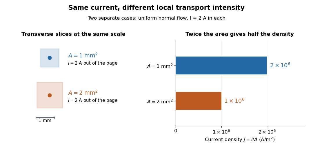
Equal electric current through different wire cross-sectional areas gives different current densities
. Both cases carry with uniform normal current density. The transverse slices use the same spatial scale; the bars compare . Source. Details.For a toy electron transport model, stipulate mobile electron number density and drift velocity , with the positive unit normal . Each electron has electric charge , where the elementary charge is exact in SI. These are defined model inputs, rather than measured parameters of a particular material. [ref] The current density and its magnitude areFor wire cross-sectional area and constant transport over time , this givesThe two minus signs make conventional current point opposite to the electron drift velocity. A small drift velocity can carry an appreciable electric current because many charge carriers contribute; it does not specify the propagation speed of an electrical disturbance.
The wire cross-sectional area is the area of a slice perpendicular to the wire's axis. For a round wire of radius , it is . It enters both the uniform-flow formula for current density and the formula for the electrical resistance of a uniform Ohmic conductor.
A charge carrier transports electric charge by moving: electrons are one example, and ions are another. For species with number density , electric charge and mean velocity , the transport contributions add as . A stationary charged background contributes to charge density but not to this current density. [ref]
https://openstax.org/books/university-physics-volume-2/pages/9-1-electrical-current. Ling, Sanny and Moebs, §9.1: positive and negative carriers
.The drift velocity is a charge carrier population's mean velocity relative to its material's rest frame. It describes the net transport superposed on microscopic motion. For a single species, current density is ; for electrons, reverses the direction. It is distinct from the propagation speed of an electrical disturbance. [ref]
https://openstax.org/books/university-physics-volume-2/pages/9-2-model-of-conduction-in-metals. Ling, Sanny and Moebs, §9.2: drift and transport
.The mean velocity of the electron population associated with a net electric current, distinct from random thermal or Fermi motion. Its sign is opposite to conventional current for negative charge carriers. Its usually small magnitude is not the propagation speed of an electromagnetic signal in a transmission line.
For sinusoidal current density and constant carrier density , the electron drift velocity is . Its displacement has amplitude and zero net change over a full cycle. The distance accumulated by this drift alone in one cycle is . With an RMS current, . This does not measure the much larger microscopic path due to Fermi velocity and electron-phonon scattering.
A charge carrier population per unit volume or, for a sheet, per unit area. The dimensional convention and whether different carrier species are counted separately must be specified.
Charge carrier mobility is the magnitude of steady drift velocity per unit weak electric field in a scalar transport model. In the Drude model, and . The positive charge carrier mobility separates ease of motion from the sign of electric charge; its SI unit is .
A transport quantity obtained by combining longitudinal electrical conductivity and a Hall coefficient. It equals single-carrier drift mobility only under the corresponding one-carrier and scattering assumptions. This does not independently determine effective mass and scattering time.
The positive hole mobility is the magnitude of an electron hole's weak-field drift velocity per unit electric field. In an isotropic relaxation-time model, , and its contribution to electrical conductivity is . The sign is opposite to an electron's drift because the electron hole has positive charge.
The positive electron mobility relates the drift velocity of conduction electrons to an electric field: . In the isotropic Drude model, , where is the momentum relaxation time and the band effective mass. The minus sign describes negative charge; the electron mobility itself is positive.
A current dipole idealizes a localized impressed electric current density by the displayed Dirac delta function distribution. Its moment has units of current times length. In a homogeneous volume conductor of conductivity , its primary electric potential is .
A radial current dipole has moment parallel to its displacement from the sphere centre. The Sarvas formula gives identically zero exterior magnetic field for such a source in a spherical volume conductor model, although its electric potential need not vanish. This is a nonuniqueness mechanism for the inverse problem in magnetoencephalography.
The four-current combines charge density and current density into the four-vector . With , its four-divergence vanishes by the charge continuity equation: . It is the source in the covariant Maxwell equations.
A surface current density is electric current per unit transverse length confined to a surface. Integrating a thin layer's current density through its thickness gives .
A current sheet idealizes electric current as supported on a surface. It produces a jump in the tangential magnetic field.
Two broad perfect conductors of width , separated by gap , carry opposite steady electric currents and connect through a terminating resistor . Away from edges, Ampère's circuital law and the superposition principle give gap magnetic field magnitude . Each conductor is an equipotential, and Ohm's law sets their electric potential difference to . Planar symmetry and charge-free Gauss's law then give uniform gap electric field magnitude . Injection parallel to the upper current makes the electric and magnetic Lorentz forces opposite. Their cancellation selects speed independent of nonzero electric charge and of operating current; nonrelativistic kinetic energy is .
The Lorentz force per unit area on an ideal current sheet is computed using the mean of its limiting magnetic fields. The sheet's own local magnetic field is equal and opposite on its two sides and cancels in this mean. Equivalently, integrate the Lorentz force density through a thin regularized layer: its self-field contribution averages to zero, leaving the external field acting on the surface current density.
A surface current density concentrated on an interface creates a discontinuity of tangential magnetic field. Let the unit normal point from side to side . In SI units, the microscopic Ampere-Maxwell law givesHere the surface current includes both free current and bound current. An infinitesimal rectangular integration loop straddling the sheet derives the tangential jump. The no-monopole equation separately gives .
In a macroscopic material description, the magnetic field intensity instead satisfiesWriting a jump in using only free current without accounting for magnetization would mix these two descriptions. In Gaussian units, the total-current magnetic-field jump is .
For an isolated uniform sheet in vacuum, reflection symmetry givesFor example, current along on gives a field along above the sheet and below it. The directions agree with the right-hand rule.
For a thin layer with essentially uniform tangential electric field, integrating electrical conductivity through its thickness gives the sheet conductivity tensor . The two-dimensional form of Ohm's law is , with surface current density . Its SI unit is : amperes per metre divided by volts per metre. When response is the same in every in-plane direction, the sheet conductivity reduces to a scalar ; for uniform bulk electrical conductivity and thickness , .
A line current idealizes an electric current as flowing along a curve; its current-density volume integral reduces to along that curve.
Electromotive force is the driving work per unit electric charge around an electrical circuit, measured in volts, despite its name containing "force". For a stationary loop its electromagnetic contribution is ; for a moving electrical conductor, include the motional electromotive force. A nonzero closed-loop line integral of the electric field cannot be represented by a single-valued electric potential alone. An electromotive force specifies the drive; the resulting electric current also depends on the electrical resistance and self-inductance. [ref]
https://www.feynmanlectures.caltech.edu/II_17.html#Ch17-S1. Feynman lectures, II.17.1: emf as a circuit integral
.Motional electromotive force is the contribution from an electrical conductor moving with local velocity through a magnetic field. The cross product comes from the magnetic part of the Lorentz force. For a straight rod of length , perpendicular to both its velocity and a uniform magnetic field, its magnitude is . The sign depends on the direction of integration along the rod. [ref].
For a computed example, take , velocity to the right, and magnetic field out of the page. The rod lies along . ThenPositive electric charge is driven downward. For an isolated rod after charge separation has equilibrated, inside it, and the electric potential difference is ; the bottom is positive. This open-circuit statement does not imply a sustained electric current.
Close the rod's path with stationary U-shaped rails and an electrical resistance at the left. With out-of-page unit normal, the positive loop direction is counterclockwise, hence upward along the rod. If the rod's horizontal position is , the enclosed area is and the external magnetic flux is . ThusHere the resistive approximation neglects self-inductance. The negative electric current is clockwise, downward along the rod, consistent with the charge-separation calculation and Lenz's law.
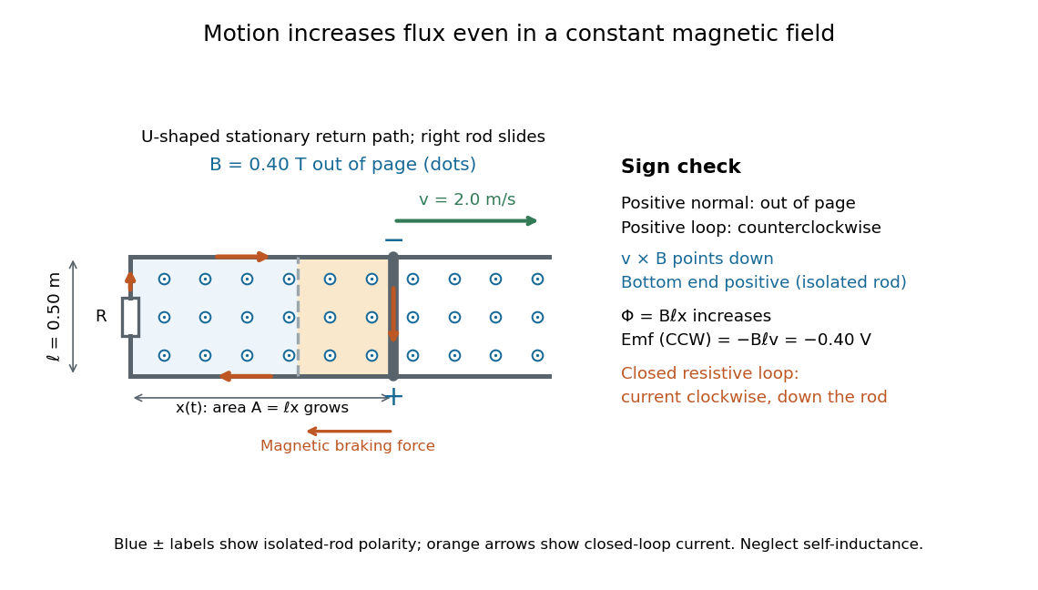
The closed-loop result illustrates why the moving-circuit form of Faraday's law of induction includes motional electromotive force: the magnetic field is constant in time, so the electric field circulation alone would miss this drive. Its mechanical consequence is electromagnetic braking of a sliding rod.
A vertical field linking a conducting loop on an incline contributes flux . For zero resistance and zero initial current, flux conservation gives . The uphill magnetic force component then makes the downhill coordinate oscillate about . Release from first stops at , not at the force-free point . The energy is stored in the inductor, not dissipated.
For positive loop resistance, coupled mechanical and circuit equations relax toward constant sliding speed on sufficiently long rails. The steady current balances the downhill gravitational force, and motional electromotive force balances the resistive voltage. The undamped zero-resistance limit has no relaxation, so its late-time limit is singular.
For laboratory velocity and field , and . Their powers are opposite. The field-dependent guide-reaction power is ; the total ideal radial reaction for bead mass and constant expansion speed additionally contributes the ordinary centripetal term .
A conducting rod sliding on rails separated by in a transverse magnetic field has induced current magnitude when self-inductance is neglected and resistance is . The Lorentz force opposes motion with magnitude , so free motion decays exponentially on the displayed time constant. Joule heating integrates to the rod's lost kinetic energy. Current direction follows the Lenz's law.
For a smoothly moving circuit and a divergence-free magnetic field, the magnetic flux derivative is . The minus sign follows by orienting the swept side surface compatibly with the two spanning surfaces. Combining this transport identity with Faraday's law yields the moving-loop electromotive-force law.
For an ohmic element, electrical resistance is and conductance is its reciprocal . They describe the same voltage-current response using reciprocal units. The relation is Ohm's law.
For an ohmic element with finite nonzero electrical resistance , its electrical conductance is : an electric potential difference drives electric current . Greater positive electrical conductance means a greater electric current for the same positive electric potential difference. Electrical conductivity is instead a bulk material coefficient relating current density to electric field.
The siemens, symbol , is the SI unit of electrical conductance and electrical admittance: . A conductance of corresponds to resistance for an ideal resistor.
The same unit can describe a complex electrical admittance in a sinusoidal experiment; that value includes a reactive part as well as conductance. For a uniform conducting sample, electrical conductivity instead has units because the conversion from material response to conductance also involves sample area and length.
Electrical resistance measures the electric potential difference needed to drive a given electric current through a component. For an Ohmic conductor under fixed material conditions, is constant and Ohm's law gives . The SI unit is the ohm, . At a fixed positive electric potential difference, increasing electrical resistance reduces electric current. Electrical conductance expresses the same response reciprocally. [ref]
https://openstax.org/books/university-physics-volume-2/pages/9-3-resistivity-and-resistance. Ling, Sanny and Moebs, §9.3: resistance and its unit
.For a straight uniform wire at rest, with constant electrical conductivity , length and wire cross-sectional area , the uniform Ohmic conductor model givesThe electrical resistivity characterizes the material; electrical resistance also includes geometry. Doubling length doubles , while doubling wire cross-sectional area halves , with material and temperature fixed. The uniform-field assumption includes insulated sides and equipotential end faces, as explained in uniform current in a straight homogeneous wire. [ref]
https://openstax.org/books/university-physics-volume-2/pages/9-3-resistivity-and-resistance. Ling, Sanny and Moebs, §9.3: wire geometry and resistivity
.As a defined wire example, take , and . Then ; applying electric potential difference drives electric current . With the same length and material, a second wire of wire cross-sectional area has and carries at that same electric potential difference. Fixing electric potential difference here differs from fixing electric current in the current density comparison: stating what is held fixed is essential.
The fractional change in electrical resistance per unit temperature change, with geometry and other conditions specified. For a small interval around , . Low is useful in stable resistors.
The continuum spreading resistance for current entering a circular aperture of radius from one uniform semi-infinite reservoir of electrical resistivity is . Two symmetric reservoirs contribute in series with a cylindrical pore resistance . Unobstructed access is not the same as zero spreading resistance; molecular-scale pores also require non-continuum transport physics.
The scale . Spin degeneracy perfectly transmitting channels instead have conductance . Suppressing charge fluctuations in a simple tunnel-island picture requires nanowire junction resistances large relative to .
Electrical resistance introduced by a connection between conducting regions. Interface chemistry, contact geometry and microscopic barriers can dominate over the bulk resistance of the connected materials. Four-terminal measurements help separate contact drops from the resistance of a test section.
The resistance per square of a uniform thin conducting sheet. For bulk resistivity and film thickness , and a rectangular stripe has . The number of squares is dimensionless and independent of an overall change of lateral scale. Networks and grids use an effective sheet resistance that may depend on finite-size connectivity and contacts.
A change of electrical resistance associated with an applied magnetic field, with material, temperature, measuring electric current and preparation specified. The response can depend on magnetic history as well as the instantaneous field. A magnetoresistance measurement therefore compares defined states, rather than treating every material as a single-valued function of field magnitude.
A large field-induced resistivity reduction in correlated magnetic materials. Double exchange links carrier mobility to spin alignment, while lattice coupling, localization and competing phases can magnify the response.
A junction with magnetic electrodes separated by a thin insulating barrier. Spin-dependent tunnelling can make resistance depend strongly on the relative electrode magnetizations.
tunnelling magnetoresistance is the dependence of a magnetic tunnel junction's electrical resistance on the relative magnetizations of its electrodes. A common convention is , where the subscripts denote antiparallel and parallel alignment. Its magnitude and sign depend on effective spin-polarized transmission through the particular interfaces and barrier.
Assume spin-conserving, low-voltage tunnelling and a spin-independent matrix element. Then parallel conductance is proportional to , while antiparallel conductance has the crossed products. Define . The two conductances are ; taking their reciprocals and using the resistance-ratio convention proves the displayed formula. Orbital filtering and interface-dependent matrix elements can invalidate a bulk-density-of-states estimate.
If one temperature-dependent relaxation scale controls a fixed carrier population and fixed orbital geometry, the magnetoresistance ratio can collapse onto a function of . This is Kohler's rule. For the equal-mobility compensated two-carrier magnetoresistance model, and . Therefore plotting against gives a common straight line of slope . A collapse tests the scaling relation; it does not by itself prove this particular microscopic carrier model. Multiple independently varying scattering times or carrier populations can spoil it.
Consider isotropic electrons and electron holes with equal density , charges , equal positive charge carrier mobility , and single-species zero-field electrical conductivity . In a transverse magnetic field, opposite Hall conductivity components cancel, while diagonal components add to . Inverting gives and . Its large-field growth is . The total zero-field resistivity is , half the single-species resistivity; confusing these quantities introduces a factor-of-two normalization error.
Giant magnetoresistance connects the relative magnetizations of adjacent magnetic layers to their electrical transport. In a suitable magnetic-metal/nonmagnetic-metal stack, aligning the layers can leave one spin channel with an easy conducting path through both magnetic layers; opposite alignments make each channel encounter a more resistive layer. Albert Fert's account traces the spin-dependent-conduction idea to Nevill Mott and distinguishes the later device geometries.[ref]
Nobel Lecture: Origin, development, and future of spintronics by Albert Fert. pp.1517–1520, spin-dependent conduction and CIP/CPP geometry
The beauty is that a magnetic arrangement becomes an electrical readout. Preparing reproducible layers, establishing their magnetizations, and measuring electrical resistance are separate parts of that inference. The Fe-Cr giant magnetoresistance experiments show how those parts were joined; the two-current resistor model isolates a simple transport mechanism under stated assumptions.
When spin-flip scattering is weak, two spin populations have separately defined current responses and share a terminal electric field. Their electrical conductivities add: , so . Spin-dependent band structure and scattering set the channel parameters; being the majority population does not universally imply lower channel resistivity. The model is named for Nevill Francis Mott and is the independent-channel basis for many giant magnetoresistance models.
A channel's electrical conductivity weights its density of states by squared velocity and the transport momentum relaxation time. In an elementary spin-conserving – scattering model, , so available heavy final states can reduce the current carried by light states. Band filling, defects and interfaces affect the asymmetry; total spin population alone does not determine its sign. A density-of-states sketch without scattering matrix elements is not a universal transport prediction.
The 1988 study grew alternating iron/chromium layers by molecular beam epitaxy on gallium arsenide. Magnetization and torque measurements tested the magnetic configuration. An AC electrical resistance measurement passed electric current along the layers while the applied magnetic field changed. Comparing field directions and spacer thicknesses linked the resistance decrease to magnetic saturation. Electron microscopy and surface analysis checked layer formation, while leaving atomic-scale interface roughness unresolved.[ref]
Giant Magnetoresistance of (001)Fe⁄(001)Cr Magnetic Superlattices by Mário Norberto Baibich and others. pp.2472–2474, preparation, Figs.1–3 and interface limits
The independent Jülich study used four-terminal sensing on epitaxial Fe/Cr/Fe strips. A single iron film supplied an anisotropic magnetoresistance comparison. Magneto-optic Kerr effect signals and Brillouin light scattering from spin waves identified the layer alignments, rather than inferring them from resistance alone. Field scans along different magnetic axes connected the optical signatures to the resistance changes.[ref]
Enhanced magnetoresistance in layered magnetic structures with antiferromagnetic interlayer exchange by G. Binasch and others. pp.4828–4830, four-point method, reference film and Figs.1–2
Peter Andreas Grünberg's retrospective explains why the preceding interlayer exchange coupling measurements mattered: coupled spin wave modes supplied signatures of magnetic alignment before that alignment became an electrical signal.[ref]
Nobel Lecture: From spin waves to giant magnetoresistance and beyond by Peter Andreas Grünberg. pp.1533–1535, coupled modes and antiferromagnetic interlayer exchange
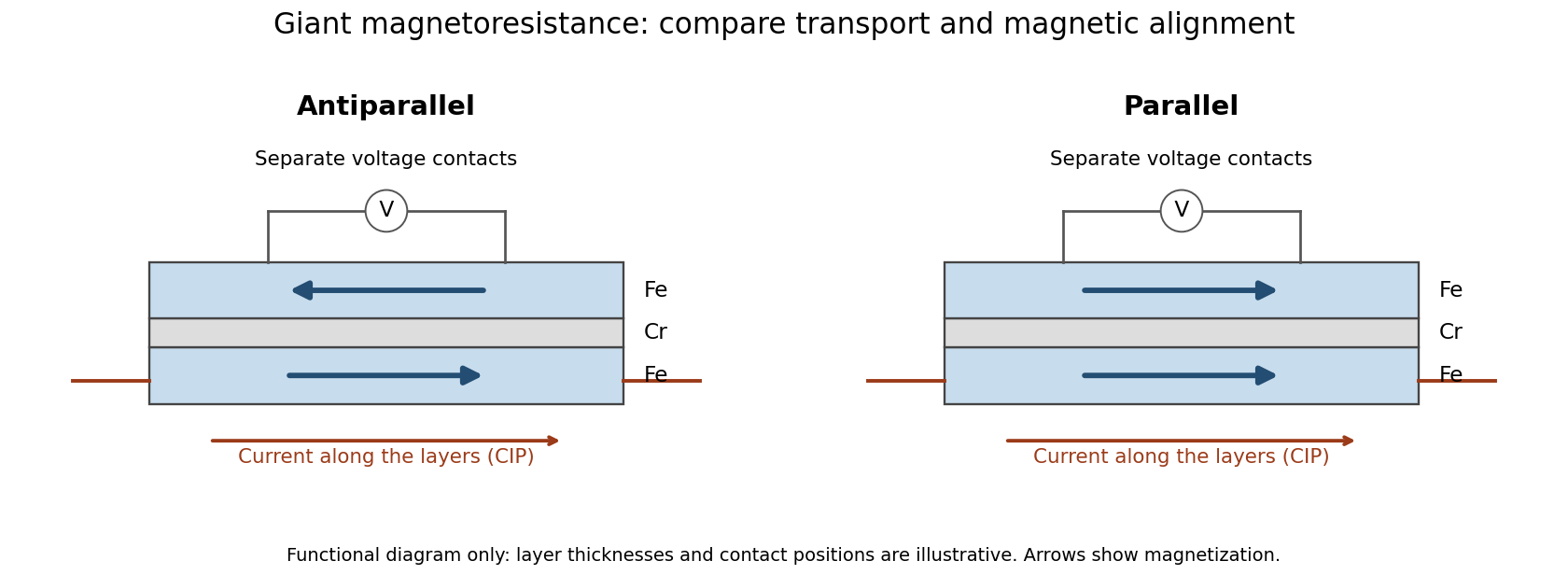
Current along a magnetic multilayer and an independent check of layer alignment
. Original functional illustration of current-in-plane transport and a generic four-terminal readout. Two idealized magnetic configurations are shown; dimensions, contact positions and layer count do not reconstruct either historical specimen. Optical probing supplies alignment information independently of the electrical signal. Source. Details.A resistance curve alone does not reveal the microscopic direction of every magnetic layer. The optical measurements add a different observable, while the reference film tests an orientation-dependent response that can occur without a multilayer. Sample preparation and cross-checks therefore belong to the physical explanation.
The measuring electric current flows along the layer planes. This is the geometry of the Fe-Cr giant magnetoresistance experiments. Scattering and current paths through an extended stack require a transport description; treating successive layers as ordinary series resistors would not follow from this geometry.
Articles were limited to the first 100 out of 171 total.
Articles by others on the same topic

Electric current is the flow of electric charge in a conductor, typically measured in amperes (A). It represents the movement of electrons through a material, and this movement can occur in various forms, such as direct current (DC), where the flow of charge is uniform and directional, or alternating current (AC), where the flow periodically reverses direction. In a circuit, electric current is driven by a voltage difference (potential difference) created by a power source, such as a battery or generator.



In the context of Maxwell's equations, it is vector field that is one of the inputs of the equation.
Section "Maxwell's equations with pointlike particles" asks if the theory would work for pointlike particles in order to predict the evolution of this field as part of the equations themselves rather than as an external element.
Measured in amperes in the International System of Units.