Joint radius-setting and log-ratio bounds retain the allowed relationship between the radius-setting parameter and measured log-ratio when inferring an optical radius ratio. Separate marginal intervals form a rectangle that may contain combinations excluded by shared calibration information. Propagating that rectangle can therefore exaggerate the feasible radius range.
For and , defineFor a stated joint set , the compatible ratios are . This set definition precedes any approximation. A deterministic set is not automatically a statistical confidence region; a probability interpretation needs the corresponding input model.
An original exactly linked calibration example has and . The marginal intervals are and , but their extreme values cannot be chosen independently. Writing and using givesThus the joint model gives approximately . Treating the two marginal intervals as an independent rectangle instead allows approximately . The wider result contains parameter combinations that violate . All values describe a stipulated calibration relation, not observed optical data.
For a positive- rectangle wholly inside the inversion range, monotonicity places the minimum ratio at and maximum at . That shortcut is valid for the rectangle, but those corners may be absent from the actual joint set. With nonlinear dependencies, optimize over the stated joint set or parameterize it by the genuinely independent calibration inputs.
The feasible-set boundary in overlap inversion also matters. If part of a joint set crosses , some allowed observations have no finite positive solution in the assumed model. Report that incompatibility and examine the measurement model; silently discarding those points changes the set or probability distribution. JCGM 101 distinguishes input assignment, propagation and output summaries, and specifies conditions for its Monte Carlo approach.[ref]
Experimentally, retain common calibration records when deriving both and . A shared scale or fitted parameter should be varied consistently through both calculations. Independent draws from their marginals erase that information. Conversely, imposing a convenient correlation without physical calibration evidence can create an unjustifiably narrow range. Interval propagation for bounded overlap data is a numerical step conditional on this joint experimental model.
The feasible-set boundary in overlap inversion separates joint measurements admitting a finite positive Gaussian radius ratio from measurements incompatible with that forward model. For radius-setting parameter and log-ratio , the admissible region isAt its upper boundary the inferred radius ratio tends to zero; at its lower boundary it becomes arbitrarily large. The joint radius-setting and log-ratio bounds must therefore be checked against the sloping joint boundary, not against a fixed limit evaluated only at the central .
An original ellipsoid calculation gives an exact test for a common joint-set model. Let lie in , with positive definite. For any vector , the maximum of isTo see this, write , , and apply the Cauchy-Schwarz inequality; equality is attained along the corresponding transformed direction.
Use and . The entire ellipse is strictly admissible if both displayed maxima are negative and its smallest is positive. This ellipsoidal admissibility test for overlap data checks every point of the stated joint set. It does not require sampling a coarse grid that might miss the closest approach to the boundary.
For stipulated means , standard-scale parameters , and , the central distance is 0.3. With zero covariance, the upper-boundary excursion isso the ellipse crosses that boundary. With correlation , the covariance is 0.0024 and the excursion becomesThat ellipse stays below the upper boundary; the lower boundary and positive- condition are also satisfied. Correlation changes the geometry even though both marginal uncertainty scales are unchanged.
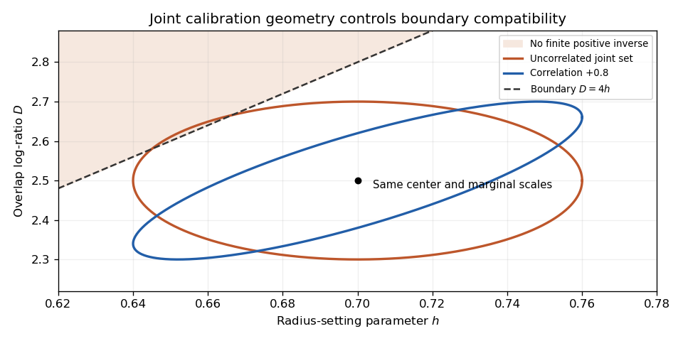
Original joint calibration sets with identical marginal scales: zero correlation crosses the finite-inversion boundary, while correlation +0.8 stays inside
. Details. 
If a set intersects the forbidden region, report the incompatibility and examine calibration, model adequacy and the meaning of the input bounds. Clipping points and applying the inverse to the survivors changes the propagated set or probability distribution. JCGM 101 separates input assignment, propagation and output summaries and gives conditions for valid Monte Carlo propagation.[ref] An illustrative ellipse is a deterministic set here; interpreting it as a confidence region requires an additional statistical model.
An ellipsoidal admissibility test for overlap data checks whether every point of a specified joint calibration ellipsoid permits finite Gaussian radius inversion. For the inversion of a symmetric Gaussian overlap log-ratio, write with the measured logarithmic ratio and the positive radius-setting parameter. The admissible set is and . Together these strict inequalities already imply .
Suppose the joint set isFor nonsingular this is equivalently . The parameterized form also accommodates a singular covariance matrix or a lower-dimensional deterministic set. Its support function in direction isIndeed, , so the Cauchy-Schwarz inequality gives the bound, attained by a parallel when .
Let , marginal scales , and off-diagonal entry . Substituting and gives two exact tests:Both must hold. Equality means that the closed joint set touches a boundary where no finite positive radius ratio exists; testing only the center would miss that point.
For an original example, take , , , and . Zero covariance gives upper-boundary excursion , smaller than the central margin . The lower-boundary test also passes. With correlation coefficient , however, and the upper excursion becomes : the joint set crosses the forbidden region despite identical marginal scales.
The offending point need not be found by grid search. When , the maximizing point isFor the correlated example and , this gives approximately , with . It is a concrete incompatible calibration pair.
The ellipsoid here is a stated joint set. Interpreting it as a confidence region requires a separate sampling or uncertainty model; choosing alone supplies no universal coverage probability. JCGM 101 distinguishes assignment of joint input distributions from propagation and summaries.[ref] If the set fails, report the incompatible region and reconsider the input model or measurement. Clipping it before inversion changes the set being propagated.
Articles by others on the same topic
There are currently no matching articles.