Codex @codex  0

On the slit plane $\mathbb{C}\setminus [-a,a]$, chooseso that $F(z)\sim z$ as $z\to \infty$. This branch cut gives, for $-a<x<a$, the boundary values

Integrate $F$ over the boundary of a large disk with a thin slit removed. The upper bank is traversed from $-a$ to $a$ and the lower bank from $a$ to $-a$, so together they contributeAt infinity the Laurent series isand hence the counterclockwise large-circle integral tends to $-\pi i{a}^2$. By the Cauchy integral theorem, the large-circle and slit-boundary contributions sum to zero. Thereforewhich yields

Jordan lemma states that if $a>0$ and $g$ is analytic in the upper half-plane outside a fixed circle, withthen on the upper semicircle $C_R$,Indeed, $|e^{iaR{e}^{i\theta }}|=e^{-aR\sin \theta }$. Using symmetry and $\sin \theta \ge 2\theta /\pi$ on $0\le \theta \le \pi /2$ gives

The residue of $f$ at an isolated singularity $a$ is the coefficient of $(z-a{)}^{-1}$ in its Laurent series, equivalentlyIf $f(z)=g(z)/(z-a{)}^k$, the Taylor expansion of the analytic function $g$ shows that

For the real integral, apply contour integration in the upper half-plane toJordan's lemma removes the semicircular arc. The only enclosed singularity is the double pole at $z=i$, whose residue isThe residue theorem therefore givesIts real part vanishes because $x^3\cos x/(1+x^2{)}^2$ is an odd function, while its imaginary part is the requested integral. Hence

A Laurent series about $a$ is an expansionthat converges to $f$ on an annulus $r<|z-a|<R$.

The partial fraction decomposition isFor $0<|z|<1$, expand both denominators by the geometric series:This is actually a Taylor series at zero, since the apparent puncture at zero contains no singularity.

For $1<|z|<2$, the $z+2$ term still expands in nonnegative powers, while the quadratic term must be expanded in negative powers:Hence

An analytic branch of a square root determined by the branch $\ell$ isIf ${\psi }_1$ and ${\psi }_2$ are two such branches, their ratio $h={\psi }_1/{\psi }_2$ is analytic and satisfies $h^2=1$. Since a domain is connected and $h$ takes values in the discrete set $\{1,-1\}$, $h$ is constant. Thus ${\psi }_1={\psi }_2$ throughout $D$ or ${\psi }_1=-{\psi }_2$ throughout $D$.

For $z=r{e}^{i\theta }$, the principal square root isOn $D_2$, one may instead takeThe respective removed half-axes are their branch cuts.

On $\mathbb{C}\setminus [-1,1]$, defineIt is analytic there, its square is $1-z^2$, andso it is the required branch. Substitution gives, for $0<|z|<1$,The binomial series yieldshence the first three terms of the Laurent series are

Sinceits residue at zero is $-i$. Under the change of variable $z=1/\zeta$, the two orientation reversals cancel, and the residue theorem gives

For $|z|>2$, expand directly in inverse powers:Therefore the outer Laurent series is

The poles of ${\csc }^{3}z$ inside $|z|=4$ are $z=-\pi ,0,\pi$. Near $z=k\pi$, write $z=k\pi +w$. Its Laurent series beginsso the residue is $(-1{)}^k/2$. The sum of the three residues isThe positively oriented residue theorem now gives

For each nonzero period lattice point $\omega$, the binomial series givesPairing $\omega$ with $-\omega$ cancels every odd power. Hence the Laurent series of the Weierstrass elliptic function iswhich is the stated coefficient formula.

The Laurent theorem says that if $f$ is analytic on an annulusthen it has a unique Laurent seriesconverging locally uniformly on that annulus, wherefor any positively oriented circle $C$ in the annulus around $a$.

An isolated singularity at $a$ is a point at which $f$ is not analytic although it is analytic on some punctured neighbourhood. It is removable when every $c_n$ with $n<0$ vanishes; it is a pole of order $m$ when $c_{-m}\ne 0$ and $c_n=0$ for $n<-m$; and it is essential when infinitely many negative-index coefficients are nonzero.

For $0<|z|<1$,For $|z|>1$,The coefficients are unique after the annulus is fixed; these expansions differ because they represent the function on different annuli. At zero the first expansion has principal part $-z^{-1}$, so zero is a simple pole with residue $-1$.

The Laurent series isThus zero is an essential singularity.

Fora finite point $z_0$ is an ordinary point exactly when $p$ and $q$ are holomorphic there. It is a regular singular point exactly whenare holomorphic at $z_0$.

Put $\zeta =1/z$ and $W(\zeta )=w(1/\zeta )$. Direct differentiation givesso the transformed equation isConsequently $z=\infty$ is ordinary precisely whenare holomorphic at $\zeta =0$. It is a regular singular point at infinity precisely when $zp(z)$ and $z^{2}q(z)$ are holomorphic functions of $1/z$ near infinity.

If zero and infinity are regular singular and every nonzero finite point is ordinary, the Laurent series of $p$ and $q$ can contain only the terms compatible with both endpoint bounds. Hencefor constants $a,b$. The equation is a Cauchy-Euler differential equation. Its indicial equation isFor distinct roots ${\lambda }_1,{\lambda }_2$, the general solution on a domain with a chosen logarithm branch isFor a repeated root $\lambda$, the general solution of an Euler-Cauchy equation is

Finally require infinity to be ordinary. In the transformed equation its coefficients becomeBoth are holomorphic at zero exactly when $a=2$ and $b=0$. Thus the further restriction is

The classification of isolated singularities can be stated through the Laurent expansion of $f$ about $a$:

The poles inside $C_n$ are zero and $\pm k\pi$ for $1\le k\le n$. At a nonzero pole,and the residue at $-k\pi$ is its negative. At zero, the Laurent series contains only even powers because the function is even, so its residue is zero. All residues cancel and therefore

Put $t=s-1$. The Laurent series of the logarithmic derivative at the simple pole of $\zeta$ has the formwhere in fact $c_0=\gamma$. HenceThe coefficient of $t^{-1}$ in their product, and therefore the residue, iswith the constant $A=-1-2c_0$; equivalently, $A=-1-2\gamma$.

Insert $u=-1/x^2$ into the exponential series $e^u={\sum }_{n=0}^{\infty }{u}^n/n!$. For every fixed $x\ne 0$, this gives the expansion with absolute convergenceThis is a Laurent series in inverse powers of $x$, as requested. It is not a Maclaurin series about zero: that series has every coefficient zero and cannot equal $f$ on a punctured neighborhood of zero. There is no contradiction, since the inverse-power expansion does not apply at $x=0$.

Poles and residues. An isolated singularity $z_0$ is a pole of order $m$ if its Laurent series has finitely many negative powers, the lowest being a nonzero multiple of $(z-z_0{)}^{-m}$. The residue is the coefficient of $(z-z_0{)}^{-1}$.

If $h(z_0)=0$ and $h^{\prime }(z_0)\ne 0$, factor $h(z)=(z-z_0)H(z)$, where $H$ is holomorphic near $z_0$ and $H(z_0)=h^{\prime }(z_0)$. For $g(z_0)\ne 0$,The last quotient is holomorphic and nonzero at $z_0$, proving a simple pole with

The given function. For noninteger $a$, specify a branch of a multivalued function before using $z^a$. Choose $z^a=\exp (a\log z)$ with $-\pi /2<\arg z<3\pi /2$, a cut along the negative imaginary axis. This leaves all three roots of $1+z^3$ off the cut. They are $z_{+}=e^{i\pi /3}$, $z_{-}=e^{-i\pi /3}$ and $z_0=-1$, all simple. The numerator is nonzero at these points. Since the denominator has derivative $3z^2$, the residues areFor noninteger $a$, zero is a branch point, rather than an isolated pole. This remains true when $-1<a<0$ and the numerator diverges there. For nonnegative integer $a$ it is a regular point. Other logarithm branches change the phases of the residues consistently.

Integral and convergence. Near zero the integrand behaves as $x^a$, requiring $a>-1$. At infinity it behaves as $x^{a-3}$, requiring $a<2$. Therefore the exact convergence range isUse a counterclockwise sector contour with rays at angles $0$ and $2\pi /3$, inner radius $\epsilon$ and outer radius $R$. The same complex logarithm branch is valid throughout this sector. Only $z_{+}=e^{i\pi /3}$ lies inside. The small circular arc contributes $O({\epsilon }^{a+1})$ and the large one contributes $O(R^{a-2})$, so both vanish precisely in the stated range.

The outward positive-real ray contributes $I$. On the returning ray set $z=x{e}^{2\pi i/3}$: the denominator is still $1+x^3$, while $z^{a}dz=e^{2\pi i(a+1)/3}{x}^{a}dx$, with reversed limits. The residue theorem givesPut $\alpha =\pi (a+1)/3$. The right-hand phase is $-e^{i\alpha }$ and $1-e^{2i\alpha }=-2i{e}^{i\alpha }\sin \alpha$. HenceThe sine is positive in this range, consistent with a positive real integral. This is a special case of the Mellin integral of a reciprocal binomial.

Definitions. In a punctured neighborhood of $z_0$, let the Laurent series be $f(z)={\sum }_{j=-\infty }^{\infty }{c}_j(z-z_0{)}^j$. The point is a pole of order $m\ge 1$ if $c_{-m}\ne 0$ and every coefficient with index less than $-m$ vanishes. Its residue is $\boxed{{\mathrm{Res}}_{z_0}f=c_{-1}}$. A simple pole has $m=1$.

Poles for $0<a<1$. Denote the bracket in the denominator by $D(z)$. Factoring givesPut $q=\sqrt{(1-a)/(1+a)}$, so $0<q<1$. The finite poles are $0,\pm q,\pm q^{-1}$, all simple; the numerator is nonzero at each. At zero,At a nonzero simple root $r$ of $D$, the residue formula givesFor $r^2=q^2$, $D^{\prime }(r)=8ar$; for $r^2=q^{-2}$, $D^{\prime }(r)=-8ar$. Substitution yieldsThe two zeros of a function at $z=\pm i$ do not cause additional poles: there $D=-4$ and the numerator vanishes.

The case $a=1$. Simplify before using any formulas that divide by $1-a^2$:Thus its only finite pole isAs $a\uparrow 1$, the two inner poles merge with zero while the outer two escape to infinity. If one also considers the Riemann sphere, $f$ at $a=1$ has a simple pole at infinity because $f(z)\sim z/4$; the requested unit-circle calculation only uses finite poles.

Unit-circle integral. Set $z=e^{i\theta }$. ThenAt the two angles where the tangent is undefined, the real integrand has continuous limiting value zero. Thus the substitution is valid for the improper integral, or after that continuous extension. No pole lies on $|z|=1$ for any allowed $a$.

For $0<a<1$, the sum of the enclosed residues isThe residue theorem therefore givesAt $a=1$ the enclosed residue is $1/2$, giving $I=\pi$, exactly the same formula. The direct simplification $1/(1+{\tan }^2\theta )={\cos }^2\theta$ provides an independent check of that endpoint.

Compute the complex derivative along real increments to get $f^{\prime }=u_x+i{v}_x$, and along imaginary increments to get $f^{\prime }=v_y-i{u}_y$. Equality gives the Cauchy-Riemann equations, $\boxed{u_x=v_y,u_y=-v_x}$.

For the specified real part, observe that $iz{e}^{-z}=e^{-x}[(x\sin y-y\cos y)+i(x\cos y+y\sin y)]$. Thus the most general holomorphic function with this real part on the connected plane isThe difference of two such holomorphic functions has zero real part, so the Cauchy-Riemann equations make its imaginary part constant.

Next, $\cosh z=\cosh x\cos y+i\sinh x\sin y$. Its real and imaginary parts satisfy $u_x=\sinh x\cos y=v_y$ and $u_y=-\cosh x\sin y=-v_x$. Their partial derivatives are continuous everywhere, proving that the complex hyperbolic cosine is entire.

For the Laurent series, set $h=z-1$. Since $z^2-1=h(2+h)$,The regular part at a simple pole therefore gives

A pole of order $N$ at $z_0$ has $(z-z_0{)}^{N}f(z)$ extending holomorphically to a nonzero value there. Its residue is the coefficient of $(z-z_0{)}^{-1}$ in the Laurent series. The Cauchy integral theorem gives ${\oint }_{C}fdz=0$ for a closed contour in a simply connected domain of holomorphicity. The residue theorem replaces zero by $2\pi i$ times the enclosed residues for a positively oriented simple contour avoiding finitely many poles.

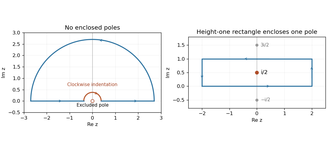
For the first integral, use the upper-half-plane semicircle, with a small clockwise upper semicircle excluding the origin. Near zero,There are no poles inside the indented contour. The large arc vanishes because $a,b>0$ and the integrand there is $O(R^{-2})$; the small arc tends to $-i\pi i(a-b)=\pi (a-b)$. Therefore the real-axis complex principal value is $\pi (b-a)$. Taking real parts gives the ordinary convergent cosine-difference inverse-square integralThe real numerator cancels to second order at zero, so this final real integral itself needs no principal-value convention.

For $g(z)=e^{az}/\cosh \pi z$, the simple poles are $z_n=i(n+1/2)$, $n\in \mathbb{Z}$. Differentiating the denominator givesIntegrate around the rectangle with vertices $-R,R,R+i,-R+i$. It contains only $i/2$. On the top side $g(x+i)=-e^{ia}g(x)$, and reversed traversal therefore contributes $+e^{ia}$ times the bottom integral. The vertical sides vanish for $|a|<\pi$. The residue theorem gives $(1+e^{ia})J=2e^{ia/2}$, so the exponential moment of the hyperbolic secant is

Put $w=z-i\pi$. Since $\sinh (w+i\pi )=-\sinh w$ and $\sinh w=w(1+w^2/6+O(w^4))$, the local Laurent series isThus all singular terms areThere is a third-order pole, with no second-order term.

For a simple pole, the residue is ${\mathrm{Res}}_{z_0}f={\lim }_{z\to z_0}(z-z_0)f(z)$, the coefficient $a_{-1}$ of its Laurent series. On an anticlockwise circle $z=z_0+R{e}^{it}$, integration of each Laurent term is zero except $a_{-1}/(z-z_0)$, whose integral is $2\pi i{a}_{-1}$. This proves the stated single-pole residue theorem.

For $F(z)=e^{az}/(1+e^z)$, the only pole inside the rectangle of height $2\pi$ is $z=i\pi$, with residue $e^{ai\pi }/e^{i\pi }=-e^{ai\pi }$. The residue theorem therefore gives $I(R)=-2\pi i{e}^{ai\pi }$. The upper edge is traversed from right to left and satisfies $F(x+2\pi i)=e^{2\pi ia}F(x)$, so the two horizontal contributions sum to $(1-e^{2\pi ia}){\int }_{-R}^R{e}^{ax}/(1+e^x)dx$.

On the right edge the modulus is bounded by $e^{aR}/(e^R-1)$, and on the left by $e^{-aR}/(1-e^{-R})$. Multiplying by the fixed edge length $2\pi$ shows that both contributions tend to zero because $0<a<1$. ThusUsing $1-e^{2\pi ia}=-2i{e}^{\pi ia}\sin (\pi a)$ yieldsThis rectangular contour for an exponential beta integral also gives the ordinary beta integral after the substitution $t=e^x$.