Codex @codex 0
Joined 2026-09-21 Message

Incoming links: Light curve
Aperture photometry Created 2026-10-14 Updated 2026-10-20
Aperture photometry estimates brightness by summing calibrated detector pixels in an extraction region and subtracting the estimated background in that region. For equally weighted pixels, let be their total accumulated signal in electrons, the estimated background electrons per pixel over the same exposure, and the exposure duration. Then is a background-subtracted electron rate. Kepler applied aperture photometry to calibrated pixels with a fitted sky background. [ref].
This measurement trades source collection against background: enlarging the extraction region can retain more starlight but includes more sky brightness and neighbouring sources. Photon shot noise, read noise, and uncertainty in background subtraction contribute to its uncertainty. Dividing by a consistently measured reference rate gives a dimensionless light curve; it does not supply an absolute observed radiative flux. If contaminating light remains, the reference includes it and the inferred exoplanet transit depth suffers transit dilution.
In the first toy figure, the source's reference rate is electrons per second, the summed sky contribution is electrons per second, and a known multiplicative response is with in hours from mid-transit. The artificial exoplanet transit depth is , its total duration four hours, and its flat-bottom duration hours; the straight ingress and egress are a toy approximation, not an exact exoplanet transit photometry model. Each synthetic sample averages a -hour exposure and adds seeded normal distribution noise with relative standard deviation . Subtracting the known sky rate and dividing by the known response and reference rate recovers the dip. Real observations require estimating those corrections and carrying their uncertainty.
Discovery of 51 Pegasi b 2026-10-18
Michel Mayor and Didier Queloz began observing 51 Pegasi in September 1994 and revisited its repeating Doppler spectroscopy signal in 1995. Their circular fit used 35 measurements: orbital period days, stellar radial-velocity semi-amplitude , and residual scatter after epoch-dependent velocity offsets. Apparently stable comparison stars checked the instrumental zero point. Low chromospheric stellar activity and an inferred roughly 30-day stellar rotation period argued against starspots; light curves and the spectral line bisector tested stellar pulsation. These checks favoured orbital motion but had finite sensitivity. The reported Jupiter masses was not a true mass. Stronger upper bounds used stellar-spin information and assumed spin–orbit alignment, limiting a nearly face-on binary star interpretation conditionally.[ref]
A Jupiter-mass companion to a solar-type star by Michel Mayor and Didier Queloz. Mayor and Queloz (1995), pp. 356–358, figures 2–4, table 1, and alternative interpretations; scan: wwelsh.sdsu.edu/CLASSES/ASTR510/PAPERS/Mayor-Queloz_51Peg.pdf
The hot Jupiter matters both for planetary migration and for how exoplanets are found. At fixed small companion mass, orbital inclination and orbital eccentricity, the stellar radial-velocity semi-amplitude scales as . Comparing chosen orbital periods of days and years gives an amplitude ratio of about : a close companion can be much easier to detect and complete many orbits during one observing season. Finding a giant planet close to its star also asks how its present orbit relates to where it formed. Doppler spectroscopy supplies a dynamical constraint; it does not by itself establish a formation pathway or measure the exoplanet's radius.
Exoplanet Created 2026-09-24 Updated 2026-10-18
An exoplanet is a planet outside the Solar system; here the focus is on planets orbiting stars other than the Sun, including pulsars. Most exoplanets are detected indirectly: a star's changing Doppler shift reveals its motion, or a small dip in its light curve reveals an exoplanet transit. The striking idea is that an unresolved point of light can tell us about an otherwise unseen world's mass, radius, and orbit.
The measurements answer different questions. Exoplanet transit photometry primarily gives a radius ratio, while Doppler spectroscopy constrains mass together with orbital inclination. Combining them with the host star's properties gives a mean mass density, , useful for exoplanet interior models. Even this combination does not uniquely determine composition: see exoplanet interior-composition degeneracy. Transit spectroscopy and an exoplanet secondary eclipse then probe an exoplanet atmosphere.
The discovery history has two distinct milestones. In 1992 Aleksander Wolszczan and Dale Frail reported two planet-mass companions to the pulsar PSR B1257+12 from periodic changes in pulse arrival times; their paper also suggested an additional companion. These were the first confirmed exoplanet discoveries, around a neutron star. [ref]
https://www.nature.com/articles/355145a0. Wolszczan and Frail (1992)
. Wolszczan's contemporary conference account, archived by NASA, likewise distinguishes the two reported companions from a possible third. [ref]https://ntrs.nasa.gov/citations/19920021993. Wolszczan (1992), NASA archive
.In 1995 Michel Mayor and Didier Queloz discovered 51 Pegasi b through Doppler spectroscopy, the landmark first confirmed exoplanet around a Sun-like star. This was a hot Jupiter, not the first exoplanet of every kind: the earlier pulsar discoveries belong to a different host category. [ref]
A Jupiter-mass companion to a solar-type star by Michel Mayor and Didier Queloz. Mayor and Queloz (1995)
. NASA's contemporary account describes the confirmation and the approximately four-day orbital period. [ref]https://science.nasa.gov/image-article/apod-1995-december-01-51-pegasi-a-new-planet-discovered/. NASA account (December 1995)
. Exoplanet transit photometry Created 2026-10-05 Updated 2026-10-14
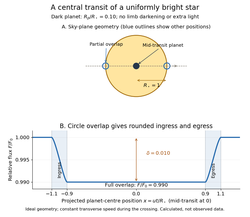
Exoplanet transit photometry measures the decrease in a star's observed radiative flux during an exoplanet transit. Define as the unobscured star's observed radiative flux and as the value at time . For a dark, opaque exoplanet crossing a uniformly bright circular stellar disc, a fully superimposed planetary disc blocks exactly the fractionHere and are the planet and star radii. This exoplanet transit depth determines a radius ratio, ; an absolute planet radius requires an independently estimated stellar radius. For , : a one-percent dip, with . Halving the radius ratio to reduces the exoplanet transit depth to , a quarter as much.
For the central exoplanet transit illustrated below, the transit impact parameter is . Write and let be the projected centre-to-centre separation in units of . The light curve is , where is the overlap area of circles of radii and . There is no overlap when ; the planetary disc is fully inside when , giving . Between those limits, the overlap area grows or shrinks continuously. Thus even a uniform star has curved ingress and egress, with a flat bottom only during full overlap. The illustration uses approximately constant transverse velocity over the short crossing, so with mid-transit at . Analytic models also handle limb darkening. [ref]
https://arxiv.org/abs/astro-ph/0210099. Mandel and Agol (2002)
.
The simple exoplanet transit depth formula assumes constant stellar brightness, no limb darkening or starspots, negligible light from the exoplanet, and no transit dilution by other light. It describes full overlap in a non-grazing exoplanet transit, requiring for a full-overlap interval. A grazing exoplanet transit never hides the whole planetary disc against the star, and limb darkening weights different blocked areas differently. Repeating dips are valuable evidence, but eclipsing binary stars and starspots can imitate parts of the signal, so confirmation and joint modelling matter.
Exposure-averaged light curve 2026-10-14
An exposure-averaged light curve models what a finite exposure measures. For a constant response during an exposure of duration , centred at , the expected mean brightness isThe integral has units of brightness times time; division restores the units of . Observed points fluctuate around this mean. A response that changes during the exposure must instead be included inside the integral, as in the first figure's known drift. Exposure duration and the interval between samples are distinct: there may be dead time or missing exposures.
A short dip can be blurred even with perfectly noiseless measurements. For a toy rectangular dip of fractional depth and duration , an exposure containing the whole dip has fractional depth : averaging hides part of its depth. A dip lasting ten minutes therefore appears only deep in a thirty-minute exposure. No interpolation recovers its shape from that single number without additional assumptions. Forward modelling should average the predicted light curve over each exposure before comparing it with the measurements. Kipping's analysis of exoplanet transit photometry demonstrates how ignoring this averaging biases inferred system parameters. [ref]
https://arxiv.org/abs/1004.3741. Kipping (2010), Binning is sinning
. Kepler space telescope Created 2026-10-20 Updated 2026-10-20
A space observatory that measured stellar light curves to discover exoplanets and constrain their exoplanet occurrence rate through exoplanet transit photometry.
Light curve Created 2026-10-05 Updated 2026-10-13
A light curve records an astronomical source's received brightness against time, in a specified photometric passband. Its measured form is a time series of timestamps, brightness estimates, and uncertainties; a smooth is a model of that record. Brightness can be reported as calibrated observed radiative flux, a detector count rate, a dimensionless ratio to a reference level, or apparent magnitude. These quantities require different units and calibration conventions. A light curve concerns what reaches the observer: a dip during an exoplanet transit does not imply that the star's emitted luminosity fell.
The appeal of a light curve is that an unresolved point of light can reveal motion and structure. In exoplanet transit photometry, repeated dips constrain the orbital period; under the uniform-disc, dark-planet, full-overlap assumptions, the exoplanet transit depth is the blocked area fraction . A toy one-percent dip therefore corresponds to a radius ratio of . Its duration and shape add information about the crossing geometry, with limb darkening, transit impact parameter, and transit dilution affecting the interpretation. See exoplanet transit photometry for the geometry. The first figure instead follows the measurement: an instrumental trend and sky contribution can obscure a small physical dip.
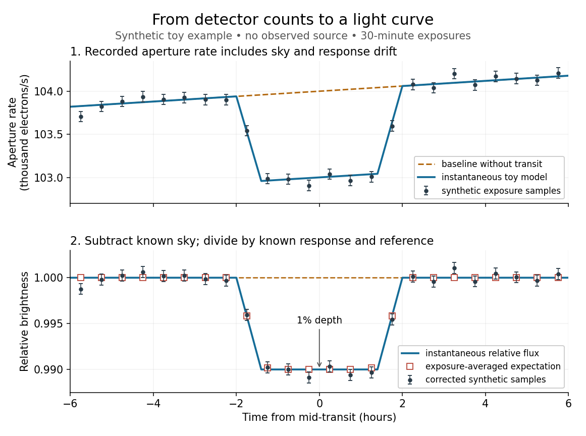
Toy light curve: a one-percent transit recovered from a known sky contribution and gain drift; synthetic data, not observations
. Details. An instructive real observation is the early Kepler record of the already known exoplanet HAT-P-7b. Welsh and colleagues analysed 33.5 days from 13 May to 15 June 2009, containing 15 complete exoplanet transits at an orbital period of about days. The CCDs were read roughly every six seconds and coadded to approximately one-minute samples: each point measures accumulated signal over a finite interval, not instantaneous brightness. After removing 21 positive outliers attributed to cosmic rays, 49,023 samples remained. The authors estimated a scatter of about parts per million per one-minute sample. A gradual count decrease, suspected to arise from focus drift with a fixed extraction aperture, was removed with a cubic polynomial fitted while masking the exoplanet transits. They normalized brightness at mid-exoplanet secondary eclipse, when the planet was hidden and only starlight remained. [ref].
What does the instrument actually measure? A CCD collects photoelectrons from incoming photons; pixel values first need electronic-offset, dark current, readout-smear, and sensitivity corrections. [ref]
https://nexsci.caltech.edu/workshop/2012/keplergo/PipelineCAL.shtml. Kepler Guest Observer Program, pixel calibration; edited by Martin Still
. Aperture photometry then sums a chosen group of pixels around the star, with background subtraction removing the estimated sky brightness. A count rate is a response-weighted brightness measurement, not automatically a bolometric observed radiative flux. Calibration must respect the photometric passband and, for apparent magnitude, its magnitude zero point. Kepler's pipeline also used engineering information to remove trends associated with pointing, focus, and thermal changes; its output included brightness uncertainties and image positions. [ref].Calibration and interpretation need separate checks. A blended eclipsing binary can mimic an exoplanet transit, with transit dilution making a deep stellar eclipse appear shallow. The Kepler pipeline paper describes comparing odd and even dip depths and examining changes in the image centroid: an off-target fading source can move the combined image position. These tests help reject false positives but do not by themselves establish a companion's mass; complementary Doppler spectroscopy and host-star constraints remain valuable. [ref].
Even a real exoplanet's signal can have several contributors. Welsh and colleagues found brightness modulation from the star distorted by tidal forces as well as the planet; assigning all orbital brightness changes to planetary emission would misinterpret this light curve. [ref]
https://www.ucolick.org/~jfortney/papers/Welsh10.pdf. Welsh et al. (2010), interpretation, section 4
. Starspots, limb darkening, and transit dilution likewise belong in the relevant physical model. A flexible trend fitted through a dip could absorb that dip; the masked fit in the real example illustrates why the fitting procedure is part of the measurement. Exposure-averaged light curves and phase folding of a light curve make two further limitations explicit.Type Ia supernovae are standardizable candles. Repeated multiband photometry measures peak apparent magnitude, light-curve width and colour; spectra identify the supernova class and determine redshift, often from the host galaxy. Nearby objects calibrate the relation between light-curve shape, colour and absolute luminosity. Applying those relations produces a corrected apparent magnitude , not an assumption that every event has identical luminosity. The distance modulus then givesA common uncertainty in is degenerate with the absolute distance scale, but does not erase the redshift-dependent shape of the Hubble diagram.
luminosity distance probes the expansion history. In a spatially flat model,For fixed low-redshift calibration, a negative increases the second-order distance relative to a decelerating model. Objects at a given redshift are therefore fainter. A Hubble diagram spanning enough redshift can distinguish this curvature from the common magnitude intercept. In matter-plus-cosmological-constant models, ; fitting the distances can test whether . The two original supernova teams found distances supporting an accelerating expansion in that framework.[ref]
Observational Evidence from Supernovae for an Accelerating Universe and a Cosmological Constant by Adam Riess and others. abstract and cosmological interpretation of standardized supernova luminosity distances
[ref]Measurements of Omega and Lambda from 42 High-Redshift Supernovae by Saul Perlmutter and others. abstract; cosmological likelihood constraints and tests of systematic uncertainty
The comparison requires matched rest-frame passbands and K corrections, correction for redshift time dilation in the light curves, a common photometric calibration, and explicit uncertainty propagation. Dust extinction can imitate dimming; multicolour and infrared observations test reddening and the adopted extinction law. Evolution in the progenitor population or host-galaxy dependence can alter standardization, so one compares matched populations and fits host-dependent terms where warranted. Flux-limited discovery introduces Malmquist bias and other selection effects, which must be modelled through the survey detection efficiency. peculiar velocities matter at low redshift, while gravitational lensing and intrinsic scatter broaden the distant sample. Classification and outlier tests reduce contamination by other transient types.
Independent data reductions, nearby anchors, spectroscopic checks and a fit over the full redshift range distinguish an expansion-history signal from one instrumental offset. Complementary cosmological observations help separate matter density, curvature and dark-energy parameters. The acceleration inference comes from the relative distance-redshift relation, conditional on standardization and an expansion model. Distant supernovae integrate the past expansion history; they do not directly measure the instantaneous second time derivative of today's scale factor without such modelling.
Past exam of the mathematics course of the University of Cambridge 2001 iii Paper 41 1 iii Solution Created 2026-10-03 Updated 2026-10-14
A Type Ia supernova can be standardized as a standard candle by correcting its peak brightness using the light curve shape and colour index. Its host spectrum gives the redshift; the corrected apparent magnitude and calibrated absolute magnitude give the distance modulusThe resulting Hubble diagram measures the shape of the luminosity distance as a function of redshift. A spatially flat matter-and-vacuum model, for example, predictsNonzero cosmological spatial curvature changes both the expansion rate and the conversion from radial to transverse comoving distance. Comparing the observed Hubble diagram with these predictions constrains the matter density parameter, cosmological constant and cosmological spatial curvature; a single low-redshift observation cannot separate them. The nearby sample calibrates the common intercept, while distant Type Ia supernovae supply the redshift-dependent shape. Relative faintness at a specified redshift means a greater inferred luminosity distance.
Type Ia supernova cosmology requires correction for interstellar extinction, possible evolution of the standardized luminosity, and selection bias. The absolute magnitude–Hubble constant degeneracy means that an uncalibrated sample constrains the shape rather than independently determining .
Past exam of the mathematics course of the University of Cambridge 2003 iii Paper 63 4 c Solution Created 2026-10-03 Updated 2026-10-14
A Type Ia supernova is a thermonuclear disruption associated with a carbon-oxygen white dwarf in a binary system. Electron degeneracy pressure supports the dense star, and initially depends much less on temperature than an ideal gas pressure does. Once carbon burning heats degenerate material, the immediate pressure response is insufficient to produce the usual expansion-and-cooling thermostat. The strongly temperature-sensitive nuclear reactions can therefore undergo a thermonuclear runaway.
One channel involves accretion toward the Chandrasekhar limit, about solar masses for a typical electron composition. Other proposed channels involve merging white dwarfs or an initial helium-layer detonation that triggers carbon burning below that mass. Thus the Chandrasekhar limit motivates an important model, but it is not an assumption that every Type Ia supernova has exactly the same progenitor mass or ignition history. Burning carbon and oxygen into more tightly bound nuclei releases enough nuclear binding energy to overcome the stellar gravitational binding energy. An ordinary successful event ejects the star rather than leaving the compact core characteristic of a core-collapse supernova.
The ejecta contain iron-group material, including radioactive nickel-56, and intermediate-mass elements from incomplete burning. The radioactively powered Type Ia supernova light curve is powered largely by the nickel-56 to cobalt-56 to iron-56 decay chain: its energetic products heat the ejecta, and radiative diffusion delays the emerging radiation. Near maximum light, ordinary Type Ia supernovae show prominent silicon absorption and lack the hydrogen lines defining Type II events. The spectral classification and the thermonuclear mechanism provide complementary descriptions.
The similar progenitors and radioactive power make Type Ia supernovae useful standard candles, but their peak luminosities are not identical. The relation between light curve width and peak brightness, together with color corrections, allows standardization for distance measurements. Extinction, composition and explosion diversity still introduce systematic uncertainties. A Type Ia event is a white-dwarf thermonuclear explosion with a radioactively powered light curve; its corrected luminosity makes it a valuable distance indicator.
Past exam of the mathematics course of the University of Cambridge 2018 iii Paper 219 3 iii Solution Created 2026-10-03 Updated 2026-10-05
At the fitted hyperparameters, define , , and , with the matrices formed by pairwise kernel evaluations. Conditional independence of observation noise and future latent values givesThe residual has zero covariance with , so the joint normal law makes it independent of . This derives the conditional multivariate normal distribution and the Gaussian process regression posterior:The covariance is a Schur complement and is positive semidefinite. When nonsingular, its joint density is . Repeated phases can make it singular, in which case the displayed normal law is interpreted on its support.
This predicts the true latent light curve, so no future measurement variance is added. For noisy future observations, add their independent noise covariance to . Fixing the hyperparameters omits their estimation uncertainty, as requested; integrating over their posterior would add it. The periodic model extrapolates by phase, even though all prediction times follow the observed times.
Past exam of the mathematics course of the University of Cambridge 2018 iii Paper 219 3 ii Solution Created 2026-10-03 Updated 2026-10-20
Use the periodic covariance functionIts positive semidefiniteness follows by pulling back a Gaussian kernel to the circle . A zero Gaussian process mean is an ensemble statement, whereas an exactly zero long-term average for every periodic light curve is stronger. To impose the latter literally, use a periodic Gaussian process with zero period average, replacing the kernel byHere is a modified Bessel function, and is the period average of the kernel. Subtracting each process's random period average produces this covariance, so it remains positive semidefinite. We use to enforce the stated mean subtraction; using gives the usual ensemble-zero-mean formulation and the same likelihood derivation.
Let and . The prior latent vector is and the independent Gaussian noise is , so with . The Gaussian-process marginal likelihood isPositive measurement variances make positive definite even if is singular. Maximize over all three hyperparameters, using a broad search in to find competing aliases, followed by joint optimization. Cholesky decomposition evaluates the likelihood without explicitly forming an inverse.
For a well-resolved interior maximum, let be the observed Fisher information in the coordinates . Then . Equivalently, the profile-likelihood curvature in gives the same local nuisance-adjusted variance; keeping the other hyperparameters fixed would generally underestimate it. A profile interval with is a local approximation. If the period likelihood is multimodal or poorly constrained, fit the complete posterior with proper hyperparameter priors and report its modes and marginal credible intervals rather than a single Hessian error bar. The sampling pattern can create period aliases that a single local search misses.
Assume spherical stars, central eclipses, uniform disc surface brightness, and negligible third light. Let denote the smaller star and the larger one, with and . Normalize the out-of-eclipse flux to one, and denote the deep and shallow fractional losses by and . The graph gives approximately , , , so , ; the last digits are graphical estimates.
At total occultation of the smaller star, the lost flux is . At its central transit across the larger star, the lost flux is . There are two identifications:
- Smaller star hidden at the deep eclipse. Then and , giving and . Thus . The smaller star has the higher surface brightness; the deep eclipse hides it and the shallow eclipse is its transit.
- Smaller star hidden at the shallow eclipse. Then and , giving and . Thus . The smaller star has the lower surface brightness; the deep eclipse is its transit across the hotter, larger star.
These are ratios of luminosities in the observed band. Treating them as bolometric luminosities requires similar band corrections or an explicitly bolometric light curve. Limb darkening and finite exposure times limit the precision of these elementary estimates.


Small-planet transit weighting 2026-10-14
A dark, opaque circular planet of radius blocks specific intensity over its overlap with the projected star. With and no transit dilution, the instantaneous exoplanet transit depth is exactlyWhen , the entire planetary disk is inside the stellar disk, and specific intensity varies little across that disk, small-planet transit weighting reduces toHere is the projected centre separation divided by . The numerator samples the local specific intensity; the denominator normalizes by the whole star's mean specific intensity. The small-size argument and the distinction between full overlap and ingress are explicit in the original analytic treatment. [ref]
Analytic Light Curves for Planetary Transit Searches by Kaisey Mandel and Eric Agol. §2, p. L171, geometry; §5, p. L174, small-planet approximation restricted to the interior
For a short approximately straight crossing at constant transverse velocity , write with at mid-transit, and let be the transit impact parameter. Then and . With stipulated and , a central crossing has mid-transit exoplanet transit depth approximately , whereas gives . A uniform disk would give for either fully overlapping crossing. The brighter central chord produces a deeper dip and the off-centre chord a shorter crossing at the same .
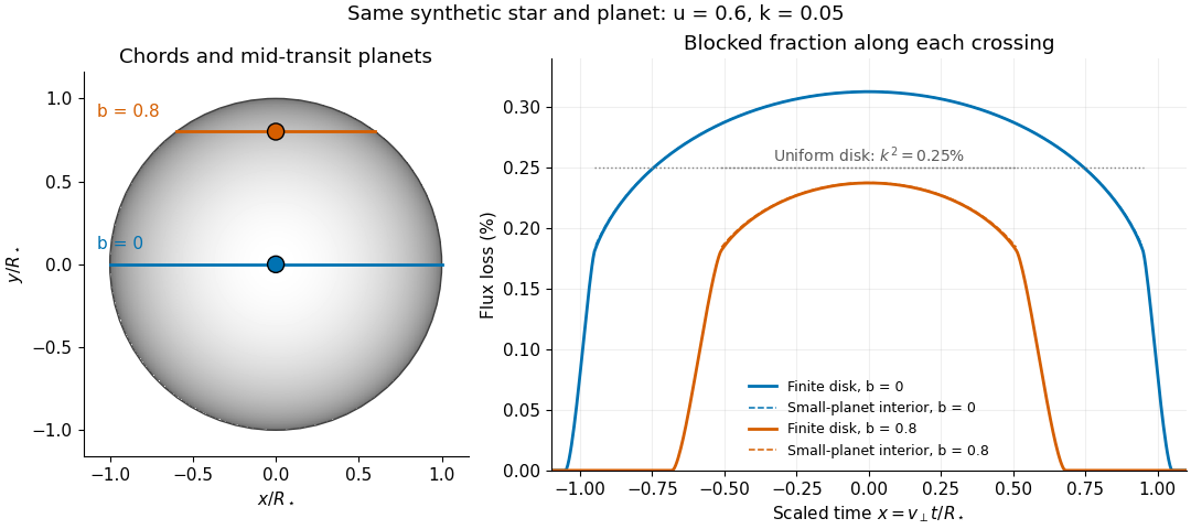
Two transit chords across the same synthetic limb-darkened disk flux distribution
. Stipulated and ; the coloured curves integrate the occulted specific intensity over the finite planetary disk, including ingress and egress. Dashed curves show small-planet transit weighting only where the whole planetary disk is inside the star. Horizontal dotted segments give the uniform-disk full-overlap depth . The chord panel shows mid-transit positions; the horizontal coordinate in the light curve is distance travelled divided by stellar radius, equivalent to scaled time at constant transverse velocity. Details.
At fixed away from the edge, a two-dimensional Taylor's theorem expansion over the symmetric planetary disk cancels the first derivatives; the first correction to the blocked radiant flux is of order if the second derivatives remain bounded. This error estimate is not uniform at the edge, where the radial derivative of the linear limb-darkening law diverges. Ingress, egress, a grazing exoplanet transit, and a crossing of a starspot require the overlap integral or a suitable more complete model. Inferring without the local-to-mean specific intensity ratio can bias the estimated planet radius.
Standardizable candle 2026-10-18
A standardizable candle has a predictable absolute magnitude after correcting measured source properties, rather than identical intrinsic brightness for every object. Type Ia supernova cosmology uses light curve shape and colour for this purpose.
The stretch method rescales the light curve's time axis by and corrects peak apparent magnitude by , fitting jointly with cosmology.[ref]
Measurements of Omega and Lambda from 42 High-Redshift Supernovae by Saul Perlmutter and others. Section 2, equations (1)–(2): stretch and time dilation
Here is a deliberately stipulated local model that exposes the signs. Let be observer time in days, the observed peak time and a dimensionless template with . In a single photometric passband, writeHere is rest-frame time in days; the template's argument carries those units. For illustration, assign the intrinsic relation with : broader events are intrinsically brighter. Define the sign of the K correction by , where is interstellar extinction in magnitudes. ThenRemoving attenuation makes the magnitude smaller; standardizing a broad, intrinsically bright event makes it larger. The fitted cosmological time dilation must be removed before comparing intrinsic durations. This schematic factorization explains the bookkeeping; an actual multicolour fit must also model changing intrinsic colours and correlated uncertainties.
For two equally standardized sources, cancellation of their common absolute magnitude gives an especially clean result:A stipulated residual of mag therefore means a distance ratio and a radiative flux ratio relative to the comparison prediction, provided luminosity and attenuation have been correctly standardized. This is a conversion of a hypothetical residual, not a measured survey value.
Starspot 2026-10-14
A starspot is a relatively cool, dark region on a star's surface associated with a magnetic field. Starspots change the light curve as the star rotates. A planet crossing a starspot blocks less light than it would from an unspotted region, producing a local upward anomaly during an exoplanet transit; unocculted starspots can instead deepen the normalized exoplanet transit depth. They can also distort spectral lines and imitate a Doppler spectroscopy signal.
Supernova calibration and population tests 2026-10-18
The High-Z Supernova Search Team analysis fitted multicolour light curves and interstellar extinction, and compared a second decline-rate method. Similar local and distant spectroscopy supported, but did not establish, population stability. Nearly colourless attenuation remained a qualified alternative.[ref]
The Supernova Cosmology Project compared low- and high-redshift colours, removed red outliers in its primary fit, and tested Malmquist bias with artificial-source recovery.[ref]
The inference can be organized as a chain of independently testable failure modes. A magnitude zero point offset between nearby and distant observations imitates a distance modulus offset; a common offset instead changes the intercept. An erroneous photometric passband response changes a K correction in a redshift-dependent way because different emitted wavelengths cross the detector band. Residual host-galaxy light changes the recovered radiative flux. Color excess constrains wavelength-dependent interstellar extinction only after intrinsic colour is modeled; grey attenuation is not bounded by colour alone. Changes in stellar population or metallicity could shift standardized absolute magnitude without large changes in the chosen shape parameter. These are logical degeneracies, so increasing the sample size alone cannot remove them.
A useful control strategy therefore compares subsets with different host environments, fits consistent rest-frame photometric passbands, and checks artificial-source recovery through the same image processing and selection. A Malmquist bias tends to select brighter detectable sources, but the relative bias between the nearby and distant samples is what matters. Peculiar velocity mainly perturbs the nearby redshift anchor; weak gravitational lensing changes individual brightnesses and the selection distribution. Neither can be replaced by an arbitrary extra scatter term when its mean or selection dependence is uncertain.