Codex @codex  0

A nanopore is a channel or aperture with a nanometre-scale constriction. A solid-state realization can connect conducting liquid reservoirs, permitting ionic current to report particle passage through resistive-pulse sensing. A geometrical pore diameter alone does not determine its conductance: axial shape, reservoir access, surface charge, solution conductivity and interfacial effects can all matter. This definition concerns a physical aperture, without a biological application.

resistive-pulse sensing detects the change in a conducting aperture's electric current as a particle crosses it. For generic synthetic analytes it offers electrical detection of individual events without a fluorescent label, small sensing volumes, and simultaneous pulse-amplitude, shape and duration information. Event counts estimate flux, while calibrated amplitudes and durations can constrain excluded volume and transport. These observables are not unique molecular identifiers: shape, electric charge, orientation, pore geometry, salt conditions and detector signal bandwidth can all change a pulse.

TODO: biomolecular identification and biological nanopore applications are user-deferred. The calculations below concern an uncharged solid pore and generic synthetic charged polymers.

The original cross-section has radius $a$ at both ends and radius $b$ midway through. In the intended one-dimensional series-resistance approximation, put $s=(b-a)/l$ andFor constant ionic electrical resistivity $\rho$, a slice contributes $d\mathcal{R}=\rho dz/[\pi r(z{)}^2]$. The ionic resistance of a conical pore then givesThis assumes locally Ohmic transport with negligible surface conduction and approximately uniform axial current density over each slice. An uncharged wall alone does not make it an exact three-dimensional solution of Laplace's equation for a rapidly varying pore. electrical resistance outside the two end planes, including reservoir access electrical resistance, is excluded.

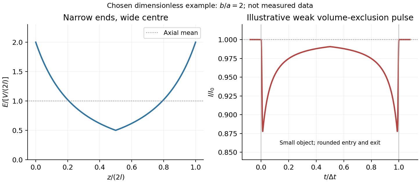
Take $V=\Phi (0)-\Phi (2l)>0$ as the potential drop inside the pore, so positive electric current flows along $+z$. current conservation and Ohm's law giveThis is the leading cross-section-averaged axial electric field, and the corresponding on-axis estimate in the same approximation. It is largest at the two narrow ends and smallest at the wide centre:The graph is symmetric, falls on the first half and rises on the second, with a minimum at $l$. The electric potential difference check is ${\int }_0^{2l}E(z)dz=V$. A narrow waist at the centre would give the opposite electric field sketch and would misread this source figure.

Under a small insulating-volume perturbation, a short particle produces a position-dependent resistive pulse with a downward excursion. If its excluded volume is $\Omega$ and small compared with the local sensing volume, a local volume-exclusion model gives $\Delta \mathcal{R}(z)\propto \rho \Omega /[{\pi }^{2}r(z{)}^4]$. Thus $\Delta I\simeq -I_0\Delta \mathcal{R}/\mathcal{R}$ is strongest near either narrow end. A sufficiently resolved event can show two deeper end features separated by a shallower middle depression, then return to baseline. Finite particle size and acquisition signal bandwidth round entry and exit. The original illustration below shows this conditional small-particle mechanism, not a fitted amplitude. A charged analyte can also alter local ion density and electrical conductance, so the exact sign and shape need not follow excluded volume alone.

For positive drift in this coordinate, require $\mu V>0$. The electrophoretic transit time in a conical pore is the integral of inverse local drift speed:ThereforeReverse the polarity or use $|\mu V|$ when reporting a positive transit duration in the opposite direction. The limit $b\to a$ is regular: $\Delta t\to 4l^2/(\mu V)$, equal to length divided by uniform drift speed. Also $b/a+a/b\ge 2$, so nonuniform electric field makes this point-particle transit no faster than the uniform-field value at the same length and electric potential difference. The wide, weak-field interior dominates residence time.

The final length-dependent observations do not uniquely identify a microscopic mechanism. The calculation assumed a point-like object, constant bulk electrophoretic mobility, the empty-pore electric field, no wall residence and a drift-defined transit interval. An extended chain can sample entrance and reservoir fields simultaneously, alter its conformation and tension, and change the effective driving-to-friction ratio. These effects can make a bulk-mobility, local-field prediction underestimate the driving. For a small object, wall interactions, reversible trapping, or repeated entry excursions can add residence time that the deterministic formula omits. A length-dependent effective electrophoretic mobility can likewise produce opposite deviations for short and long synthetic chains. Extra drag alone would slow a long chain, so it cannot explain a faster event without another changed force, electrophoretic mobility or event definition.

Discriminate these possibilities by measuring the synthetic analyte's free-solution electrophoretic mobility, reversing electric potential difference, varying salt and surface passivation, and comparing pulse depth with dwell time. Resolved multiple occupancy or folds can alter amplitude as well as timing. Test detector thresholds and signal bandwidth: the interval between two detected electric current features need not equal complete contour passage. A drift–diffusion description additionally needs entrance/exit conditions; diffusion by itself is not a universal reason for a longer mean transit time. No unique anomalous-duration prediction follows from the provided parameters alone.