Ohm's law states that an Ohmic conductor has electric current proportional to its applied electric potential difference, with constant electrical resistance under fixed material conditions:Here is the terminal electric potential difference, and positive enters at and exits at . This sign convention makes the electrical power absorbed. The straight-line relation through the origin lets one constant predict the response at many applied electric potential differences. Merely defining at one nonzero operating point does not establish Ohm's law: a component may have a ratio that varies with applied electric potential difference. Material and temperature must be specified and held fixed; many components have a nonlinear response. [ref]
https://openstax.org/books/university-physics-volume-2/pages/9-4-ohms-law. Ling, Sanny and Moebs, §9.4: Ohmic and non-Ohmic responses
.For the ideal resistor model at electric potential difference ,This power is converted to internal energy by Joule heating; a watt is a joule per second. If the model holds for time , the transferred energy is . Doubling electric potential difference doubles electric current and quadruples power for the same fixed . The model keeps material temperature fixed even while calculating Joule heating; appreciable changes in temperature may require a changing electrical resistance. [ref].
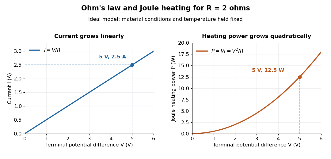
Ohm's law gives linear electric current and quadratic Joule heating power at fixed electrical resistance
. The ideal model holds fixed. At , the marked values are and . Source. Details.In 1827, Georg Ohm published his mathematical account of electrical transport in Die galvanische Kette, mathematisch bearbeitet. On printed page 36, his relation expresses electric current in terms of total driving tension and a reduced length incorporating electrical conductivity and geometry. This is historical notation: his is not the wire cross-sectional area used here, and his is not simply the wire's physical length. The striking idea is that material response and geometry can be combined into one quantity governing an electrical circuit. [ref]
https://archive.org/details/diegalvanischek00ohmgoog. Ohm, Die galvanische Kette, mathematisch bearbeitet (1827), p. 36, original edition
.Author of the 1827 treatise developing the electrical transport relation now called Ohm's law. [ref]
https://archive.org/details/diegalvanischek00ohmgoog. Ohm, original 1827 treatise
.Electrical conductivity measures the local response of current density to electric field. In the rest frame of an isotropic Ohmic conductor, the local form of Ohm's law isLarger positive electrical conductivity gives larger current density at the same electric field. It is a bulk material coefficient, distinct from the geometry-dependent electrical conductance of a whole component and from a sheet's surface conductivity. Electrical resistivity is in this scalar model. [ref]
https://openstax.org/books/university-physics-volume-2/pages/9-3-resistivity-and-resistance. Ling, Sanny and Moebs, §9.3: conductivity and resistivity
.The local and whole-wire forms fit together particularly neatly. For uniform current in a straight homogeneous wire, with length , wire cross-sectional area , constant electrical conductivity and terminal electric potential difference , the axial electric field has magnitude . ThusFor the defined electrical resistance example , , and , the local values are and ; integrating gives . One material law therefore supplies both a spatial description and a terminal relation.
The scalar form requires isotropy. In an anisotropic material the response can instead be a tensor, , and current density need not be parallel to electric field; uniaxial conductivity tensor is one existing example. These statements concern the material's rest frame. A moving electrical conductor instead uses the moving-conductor Ohm law.
In a steady series circuit, both electron and hole conventional currents contribute in the intrinsic semiconductor, while one electron population carries the metal current. Taking magnitudes along the current direction gives the displayed relation, with in the intrinsic region. The large metal carrier density can yield a much smaller drift speed despite its smaller cross-section. Interface conversion between electron and hole transport does not violate total current continuity.
Electrical conductivity arising from motion of ions. In a dilute, uncorrelated vacancy model, a mobile oxygen vacancy has effective charge and moves opposite to the oxygen ions that fill it.
With the explicitly stated convention , the tracer and collective diffusion coefficients are related by . The Nernst-Einstein relation then gives . State the convention, since reciprocal definitions can otherwise cause confusion.
The activation free-energy barrier for an ion to hop between sites. ionic conductivity also depends on the concentration of mobile defects and correlations between successive hops.
For dilute, independently migrating carriers of number density , charge and diffusion coefficient , balancing drift with diffusion gives mobility per applied force. Multiplying drift velocity by charge density yields . State which species defines and : a vacancy diffusivity must be combined with vacancy density. Correlated motion requires a correction rather than automatic use of a tracer diffusivity.
The density and diffusivity in must refer to the same carrier species and correlation convention. Oxygen vacancy diffusivity belongs with vacancy density; tracer diffusion of oxygen atoms is not automatically the vacancy diffusivity. A transport inversion may determine an effective density without uniquely determining a chemical defect concentration.
An alternating electric current and its electromagnetic field concentrate near a conductor's surface. For a local isotropic good conductor with real electrical conductivity , magnetic permeability , and , the field penetrates over the skin depth .
With fields proportional to , a homogeneous Ohmic medium obeys the displayed relation by combining the two curl Maxwell equations. The physical passive branch has . For real positive conductivity much larger than , it reduces to with skin depth . Field amplitude and intensity then decay with respective lengths and . A frequency-dependent conductivity must be retained when charge-carrier inertia matters.
A coating substantially thinner than the skin depth does not screen the substrate as a bulk conductor would. Thickness of a few skin depths suppresses the field reaching the substrate exponentially. A unique required thickness additionally needs an allowed residual field or loss criterion.
In the normal skin-effect regime of a good conductor, and the surface resistance is . For identical geometries, resistance ratios depend on the square root of magnetic permeability divided by conductivity.
For a wave penetrating a nonmagnetic good conductor in the direction with time convention , its wavenumber is , with skin depth . If , Faraday's law of induction gives . Thus the field ratio is , equal to the displayed expression. Magnetic and electric fields have equal exponential penetration lengths but a phasor phase difference ; has the positive phase relative to in this convention.
The skin depth is the distance over which a field amplitude falls by inside a conductor. In the local good-conductor limit, . Intensity then falls by over one skin depth; amplitude and intensity penetration lengths differ by a factor two.
The tensor relating local current density to electric field. Its inverse, when it exists, is the electrical resistivity tensor; sheet conductivity uses surface current density instead.
Complex conductivity relates the complex amplitudes of current density and electric field at an angular frequency in sinusoidal response. Its modulus gives the amplitude ratio, while its argument encodes their relative phase. Both the exponential time convention and whether amplitudes are peak or root mean square values must be stated when interpreting phase or average power.
Electrical resistivity is the inverse of scalar electrical conductivity in an isotropic Ohmic medium. In its rest frame, , so the electric field does work per unit volume . In Gaussian units, finite conductivity gives magnetic diffusivity ; neglecting this diffusion is a distinct approximation from neglecting electron inertia in Hall magnetohydrodynamics.
A phenomenological label for metallic responses that depart from ordinary Fermi-liquid expectations, commonly including a broad approximately temperature-linear resistivity regime in some cuprates. The observed range depends on doping, field and material. A linear law alone does not uniquely identify the scattering mechanism, and the ordinary metal's high-temperature phonon-linear resistivity is not by itself evidence of the same regime.
The resistivity tensor is the matrix relating electric field to current density in linear local transport. It is the matrix inverse of the conductivity tensor, not the componentwise reciprocal. A Hall response produces antisymmetric off-diagonal components. In a multicarrier system, the conductivities add because each species sees the same electric field; invert only after summing the species' conductivity tensors.
The residual resistivity is the low-temperature electrical resistivity remaining in a normal metal when thermally excited scattering becomes negligible. Static disorder, impurities and boundaries can relax carrier momentum without requiring a thermal population of phonons. Its value depends on sample purity and structure; a superconducting transition is a different phenomenon.
Matthiessen's rule approximates the total electrical resistivity of a metal by the sum of separate scattering contributions. For a common parabolic energy band, approximately independent scattering mechanisms give for the respective momentum relaxation times, and hence . Correlated scattering, strongly angle-dependent processes or a complicated changing energy band structure can invalidate the simple addition.
The sheet resistivity tensor relates tangential electric field to surface current density: . It is the matrix inverse of the sheet conductivity tensor, when that inverse exists. Its SI unit is the ohm, rather than the ohm times metre used for bulk electrical resistivity. With a transverse response, individual tensor components are not generally reciprocals of the corresponding sheet conductivity components.
For a spin-degenerate parabolic two-dimensional band, the Drude model gives and . Their product is the displayed mass-independent mean free path. A Fermi-surface transport interpretation requires a sufficiently degenerate electron gas; a quantum lifetime need not equal the transport relaxation time.
The in-plane dissipative response along an imposed sheet current. In an isotropic Hall system, matrix inversion gives . It is a sheet quantity in ohms, while a homogeneous strip's measured longitudinal resistance additionally includes its length-to-width ratio.
A uniaxial electrical conductivity has one distinguished direction and equal response in its orthogonal plane. Its eigenvalues are in and along , so it is invertible precisely when . For an electric field perpendicular to , the electric current density is . Positive dissipation requires both eigenvalues to be nonnegative, a physical constraint separate from algebraic invertibility. For , one has , and is equivalent to ; the conductivity then vanishes along .
An electrical conductor supports mobile charge carriers and hence an electric current under a field. In a band description, a partially filled band or available overlapping bands supply nearby accessible states. The contrast with a band insulator depends on band filling as well as spectral gaps; semiconductors provide carriers through thermal excitation or doping.
An ideal planar conductor is an equipotential boundary in electrostatics. The electric field just outside is normal to it, while the electric field inside its metal vanishes. If grounded and infinite, the method of images implements the boundary by reflected opposite electric charges.
A material whose current density is proportional to its electric field, with proportionality given by its electrical conductivity.
In a homogeneous Ohmic conductor, a steady electric current density obeys and . Uniform axial current in a straight cylinder follows if its side is insulated and its flat end faces are equipotentials. The electric potential then solves Laplace's equation with those boundary conditions, and uniqueness makes it linear in the axial coordinate. Steadiness alone does not impose these contact conditions: nonuniform end potentials can produce nonuniform current even with an insulating side. Bending also generally redistributes current; in an annular conductor the azimuthal current density is proportional to the inverse radius.
In a homogeneous Ohmic conductor, the charge continuity equation and Gauss's law imply exponential decay of the bulk charge density, . For an isolated finite body, bulk charge moves to its boundary; the accumulating surface charge density preserves total electric charge. The formula uses a constant permittivity and the corresponding free-charge convention, or for total charge in the vacuum form of Gauss's law.
A uniform cylindrical volume charge relaxes exponentially under Ohm's law and the continuity equation for electric charge. In a cylinder of radius initially carrying no surface charge, the radial conduction current deposits on its surface. Total charge per unit length remains , so the exterior radial electric field is time independent even though the interior field decays. Neglecting the deposited surface charge violates charge conservation.
The Drude model explains finite electrical conductivity by balancing charge carrier acceleration in an electric field against loss of directed momentum through collisions. Its useful surprise is that continuous microscopic motion can produce a constant macroscopic current density: the applied electric field continually restores the directed momentum lost to the material. The simplest version has one mobile species, constant number density , electric charge , mass , and momentum relaxation time , in a stationary, homogeneous, isotropic material. At zero magnetic field, its mean drift velocity and current density obeyFor electrons, with positive elementary charge , so . The electron drift velocity points against a constant electric field, whereas conventional current points along it. Random microscopic velocities can have zero mean without being zero individually; drift velocity is this population mean, rather than each particle's speed.[ref]
The same first-order linear differential equation predicts both Drude current relaxation after switching an electric field and the Drude frequency response to a sinusoidal electric field. Together they let a measured electrical conductivity be interpreted in terms of a density, a mass, and a time scale; a single constant-field measurement determines only their combination .
The original 1900 paper Zur Elektronentheorie der Metalle by Paul Drude sought a common account of electrical transport and heat transfer using mobile charged particles and ideas from the kinetic theory of gases. Its introduction, especially printed pp. 568–569, explains that comparing different transport phenomena could constrain the populations of free and bound charged particles. The modern momentum relaxation time formulation above is a useful presentation of the model, not a verbatim translation of the original notation or its historical assumptions about mass.[ref]
Zur Elektronentheorie der Metalle by Paul Drude. pp. 568–569: motivation for combining transport phenomena; OCR has spelling and formula errors
The momentum relaxation time is the exponential relaxation time of mean directed momentum after the driving electric field is removed. In the simplest Drude model, independent collisions occur with probability during a short time interval and reset the mean velocity of the collided population to zero. The remaining fraction preserves its previous mean momentum. To first order in , averaging gives . This is a population equation: it does not assert that every particle stops at equally spaced instants.[ref]
For real materials, a collision that changes a particle's direction only slightly need not erase its directed momentum, so the momentum relaxation time need not equal the time between all scattering events. This transport time is also distinct from the bulk charge relaxation time : one describes loss of directed motion, the other redistribution of charge density.
Switch on a constant electric field at . For prescribed initial current density , the exact Drude model solution is the displayed formula. For electrons, the corresponding drift velocity isStarting from zero drift velocity, the current density reaches of its limiting value after one momentum relaxation time. Switching the electric field off at instead gives for . A finite step of electric field changes the acceleration immediately but leaves drift velocity and current density continuous.
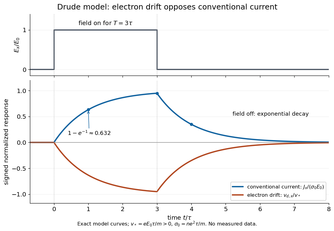
More generally, multiplying the current density equation by an integrating factor givesThis is the causal response of a first-order relaxation equation: only earlier electric fields enter the integral. It also shows why instantaneous Ohm's law is an approximation when the electric field changes appreciably during a momentum relaxation time.
Use physical electric fields and current densities , with peak complex amplitudes. After the initial transient has decayed, substitution into the Drude model equation gives the complex conductivityHere the mobile species is electrons. With the alternative convention, the denominator is and the imaginary part changes sign; the physical response is identical.[ref]
For with , the real-time current density isThus a positive argument of complex conductivity in the convention means that current density lags the electric field. At , its real part and imaginary part are both , its modulus is , and the lag is .
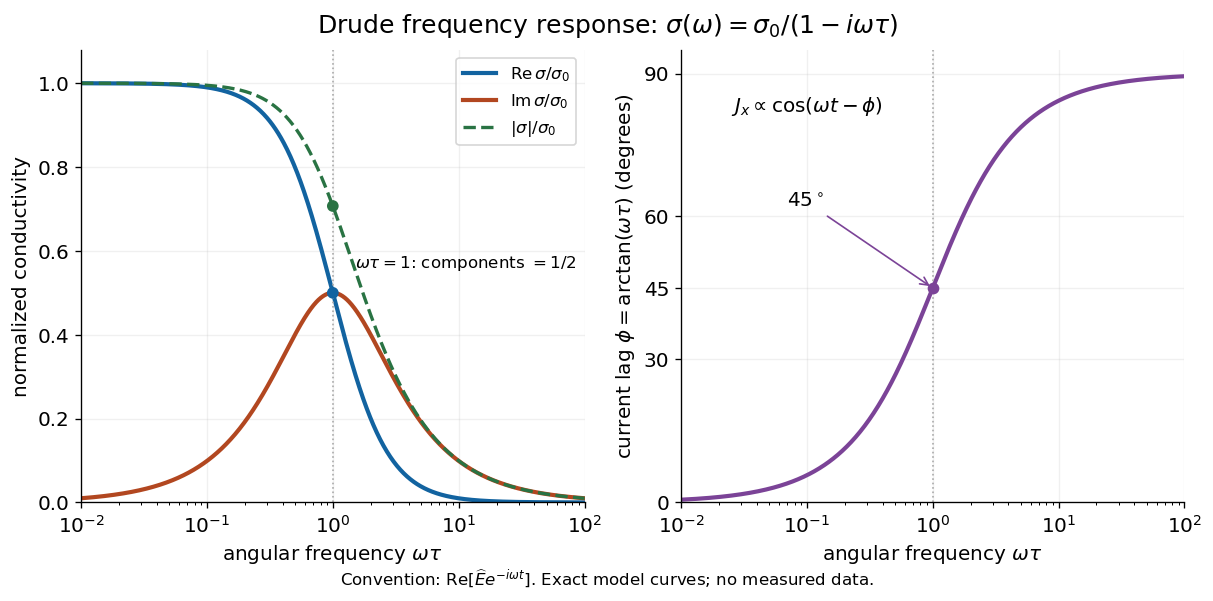
For , complex conductivity tends to the positive constant : current density nearly follows the electric field. For within this model,The current density amplitude decreases and its response becomes predominantly inertial. Average power absorbed per volume is . These limits describe the material response to a specified local electric field, not the complete electromagnetic response of a finite specimen with contacts. The Drude response has its pole at , consistent with the decaying causal response of a first-order relaxation equation.
The simple Drude model does not predict the microscopic momentum relaxation time. It neglects electronic band structure and Fermi-Dirac statistics; a useful semiclassical extension replaces by an appropriate band effective mass, but neither a single scalar mass nor one constant momentum relaxation time describes every material. Several charge carriers, energy-dependent scattering, and transitions between electronic bands can spoil the simple Drude frequency response. A successful low-angular frequency fit does not justify extrapolation to arbitrarily large angular frequencies.
For charge , field , time dependence and circular components , the active positive-frequency response is the plus component and its denominator contains . Reversing the field or exchanging helicity labels swaps the signs. A printed circular conductivity must state those conventions together.
A doped semiconductor at frequencies far below its bound-electron resonances can haveFor a weakly absorbing nonmagnetic half-space adjacent to vacuum, the normal-incidence optical reflectance is minimized near refractive-index matching, . When and is small this gives . The zero of the real part of , near , is a distinct frequency. Increasing the carrier density shifts the minimum to shorter wavelength if the carrier effective mass and background response remain fixed. With appreciable loss, the minimum must be found from the full complex Fresnel equations.
For a weakly absorbing doped semiconductor with one dominant carrier species and approximately constant background dielectric function , the Drude model gives a normal-incidence reflectivity minimum near . Thus , with and . Eliminating the plasma frequency proves the displayed mass estimate. The real-dielectric zero instead has and is the nearby screened plasma edge, so its wavelength requires a different denominator. With appreciable loss, fit the full complex Fresnel equations rather than identifying the minimum with an exactly real dielectric value.
A motivating laboratory realization is The Hall Effect and Conductivity in Germanium by Rex Tayloe. The handout specifies a germanium sample holder with temperature and magnetic field control, a low-voltage supply, digital meters, and a current-reversing switch. Measure the sample dimensions, map the contacts, and establish the directions of electric current, magnetic field, and transverse voltage. At fixed temperature and zero magnetic field, sweep positive and negative electric currents and record longitudinal electric potential differences. A straight voltage-versus-electric current relation tests Ohm's law; sample geometry converts its slope to electrical resistivity. For the Hall effect, minimize the zero-field transverse offset and measure transverse voltage at all four combinations of and , repeating for several electric currents. The readouts test longitudinal proportionality, transverse polarity, and transverse proportionality to electric current. These are protocol instructions, not reported measurement outcomes.[ref]
The Hall Effect and Conductivity in Germanium by Rex Tayloe. pp. 1–3, Equipment, Fig. 1, and At room temperature: conductivity sweep and four polarity combinations
For interpreting such measurements, an ideal uniform bar of wire cross-sectional area with longitudinal sensing contacts separated by gives . Four-terminal sensing suppresses voltage drops in current contacts when the voltage meter draws negligible electric current; it does not fix uncertain dimensions or a nonuniform current density. Reverse electric current and use to reject a constant voltage offset. Keep temperature stable, allow the current density to settle, and reduce electric current to test for Joule heating. Those are controls for interpreting the material coefficient, rather than reasons to assume every measured curve is linear.
For the transverse measurement define , , width along , and thickness along . Define , so givesExtract the part odd in both electric current and magnetic field usingThis combination rejects a constant offset and longitudinal pickup even in magnetic field. It cannot reject another signal with the same two reversal symmetries. Check field polarity and magnitude independently; a sign error in the contact map changes the inferred Hall coefficient.
For one Drude model species in transverse open circuit, the steady Lorentz force balance is with . Its component gives . ConsequentlyLongitudinal electrical conductivity and the Hall coefficient therefore separate number density from charge carrier mobility in this single-species model. Inferring a momentum relaxation time additionally requires an appropriate mass. A constant-field longitudinal measurement alone cannot supply all three.
A Hall coefficient is not universally the reciprocal of signed number density. For example, adding independent electron and electron hole contributions with densities and positive charge carrier mobilities in the weak-magnetic field limit givesThe Hall coefficient can vanish even while electrical conductivity is positive, and its sign weights charge carrier mobility as well as number density. The germanium handout explicitly asks students to track possible transverse sign changes with temperature; it does not establish a universal single-carrier interpretation. Real electronic band structure and unequal scattering also limit that interpretation.[ref]
The Hall Effect and Conductivity in Germanium by Rex Tayloe. p. 1, Experiment, and p. 3, As a function of temperature: tracking carrier sign and Hall-voltage sign changes
The Drude model relative permittivity is . At frequencies large compared with the collision rate but below , its leading real part is negative and the physical spatial wave-number branch has positive imaginary part. The field therefore decays into the conductor; close to the threshold the full complex response must be retained.
Joule heating is the dissipative conversion of electrical work into internal energy in an electrical conductor. In a metal, the electric field supplies energy to charge carriers, which transfer it to the material. This makes an immersed resistor a useful calibrated heater and makes electrical resistance a source of losses in wiring. Wind-driven electric currents are a proposed source of heating of an inflated giant planet.
For a stationary, purely resistive Ohmic conductor, use the passive sign convention: is the terminal electric potential difference from the entry to the exit of positive electric current . The absorbed electrical power and Ohm's law giveThe last two expressions assume at the relevant material temperature. For constant electrical resistance and electric current over a duration , the dissipated energy is ; otherwise use . In SI, .[ref]
Absorbed electrical power is more general than Joule heating: a capacitor can store energy, a battery can change its chemical energy, and an electrical circuit can deliver mechanical work or emit light. Even a heated resistor need not show an indefinitely rising temperature: in a thermal steady state, its dissipated power leaves by heat transfer. With the heater inside a calorimeter boundary, electrical input crosses as work; the subsequent heat transfer to the room is a different term in the first law of thermodynamics.
A resistor at fixed temperature and unchanged thermodynamic state has no net entropy accumulation. Electrical work becomes heat at rate , which is exported to the thermostat. In the ideal work-source model the surroundings gain entropy at rate , equal to the total entropy production. Additional losses inside a real power source add to this idealized budget.
Whether increasing electrical resistance increases Joule heating depends on what the supply holds fixed. Consider separate ideal resistor experiments with and , each maintained at its specified temperature. At fixed electric current , doubling changes the required electric potential difference from to and doubles power from to . At fixed electric potential difference , doubling halves electric current from to and halves power from to . These are stipulated model values, not measured data.
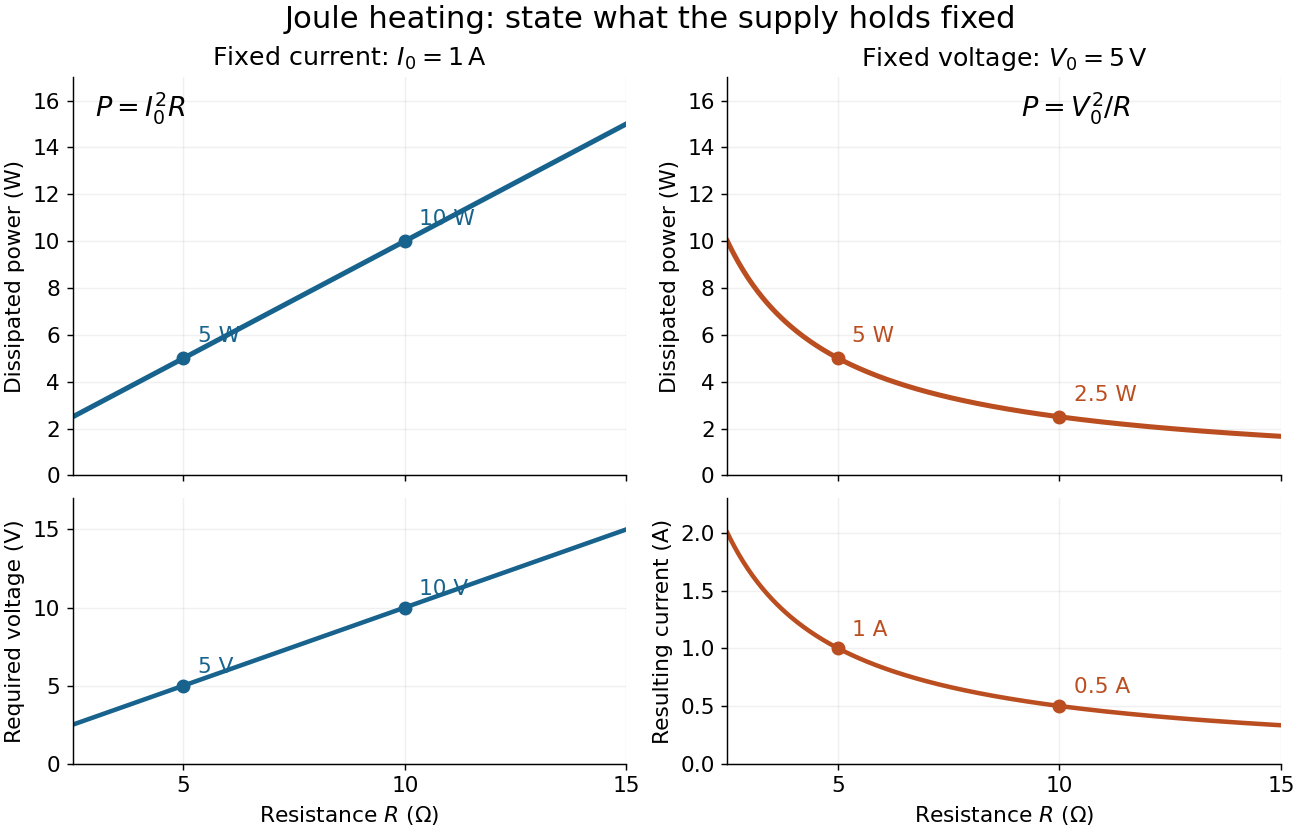
Increasing electrical resistance has opposite effects on Joule heating under fixed electric current and fixed electric potential difference
. Original calculated comparisons, with on the left and on the right. The marked and cases are separate ideal experiments. Each lower panel shows the companion quantity that changes when the supply holds the other quantity fixed. Details.The comparison also predicts feedback when a particular resistor's electrical resistance rises with temperature: a supply maintaining electric current increases its heating power, whereas one maintaining terminal electric potential difference reduces it. Predicting the actual temperature still needs the material response and its heat transfer to the surroundings; a nominal supply setting does not establish which drive is actually constant at the resistor.
The electric field does work on matter at local power per volumeHere is current density and the dot product includes the relative direction. Positive means energy passes from the field to matter; negative means matter supplies energy to the field. In general this is a work rate, not automatically an irreversible heating rate.[ref]
For a stationary isotropic Ohmic conductor with real scalar electrical conductivity , local Ohm's law gives . Thus the local Joule heating rate isThe electrical resistivity has units , and electrical conductivity has units . These formulas use the material's rest frame and dissipative conduction current density. Moving media, complex conductivity, and additional storage or transport processes require their appropriate energy balance rather than this scalar substitution.
For uniform current in a straight homogeneous wire of length , wire cross-sectional area and constant electrical conductivity, , and . The volume integral recovers terminal power:As a numerical check, the wire already used in electrical resistance has , , and . It gives , and , agreeing with and . Concentrating the same electric current in a smaller wire cross-sectional area therefore raises the local heating rate if electrical resistivity stays fixed.
A long wire with uniform current density generates uniform heat per volume . Radial steady conduction obeys . Regularity at the centre removes a logarithmic solution, leaving the displayed parabolic temperature excess relative to the surface. Conductivity, electrical conductivity and current density are assumed constant.
The surface flux of a uniformly heated cylinder is . Equating it to the Newton-cooling flux gives the displayed surface temperature. The full temperature profile adds the internal parabolic excess to this surface value. Electrical power per length equals the surface heat loss per length in steady state.
An electrical calorimetry experiment asks whether a measured electrical work input accounts for a measured warming. The University of Iowa's demonstration uses an insulated flask containing water, an immersed heater, a thermometer, electrical meters and a timer. Its procedure compares the duration, electrical readings and temperature rise. The following low-power measurement design and synthetic readout develop that idea; they are not measurements reported by the demonstration. [ref]
5F15.10 - Electrical Equivalent of Heat by University of Iowa Department of Physics and Astronomy. Equipment and Procedure: insulated flask, immersed heater, thermometry, electrical meters and timed warming
Use a covered calorimeter with weighed water, an immersed resistor, a calibrated thermometer and gentle stirring. Put an ammeter in series with the heater branch and a high-input-electrical resistance voltmeter across the immersed resistor's terminals. Record , , temperature and room temperature before, during and after switching the heater on. Measure the electric potential difference at the heater, rather than at the supply: lead and contact electrical resistance outside the receiving boundary can consume power that never reaches the water. Account for voltmeter loading if the ammeter also includes the sensing branch's electric current.[ref]
The electrical readout gives operating electrical resistance when , and power . To test Ohm's law, obtain several pairs at the same temperature; one ratio alone cannot establish a linear response. For small electrical resistance, use four-terminal sensing to exclude lead drops and reverse electric current to test stable offsets from the thermoelectric effect. Use brief low-power resistance measurements if the intended result is the unheated value: the test itself causes Joule heating.
For a covered assembly at approximately constant pressure, with negligible evaporation, negligible endpoint mechanical energy changes and no phase transition, takeHere is the water's specific heat capacity at constant pressure, is the participating vessel, heater and sensor heat capacity, is signed outward heat leakage, and is stirring work entering the assembly. The storage term approximates its enthalpy change; for a rigid fixed-volume receiver use the corresponding heat capacity at constant volume. Calibrate independently if the purpose is to test electrical input against thermal storage. Using the same heating run to define and then claiming it verifies the equality would be circular.
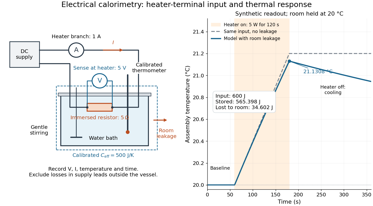
For the synthetic trace, stipulate , , , , room temperature , and loss coefficient , with negligible stirring input. The heater runs for , beginning at room temperature. The calorimeter heat-loss correction model isIt predicts , , storage and outward loss . Neglecting leakage undercounts deposited energy by about ; assuming no loss predicts . After switching off, the excess temperature undergoes exponential decay with time constant . A cooling slope can estimate only with known and a credible single-temperature model.
Controls separate causes of a temperature rise. Check the electrical meters' zeros and thermometer calibration; keep water mass, immersion, lid and stirring fixed between runs. Record a heater-off stirred baseline to estimate sensor drift and stirring input. Repeat cooling runs over the same temperature range to estimate environmental heat transfer; a baseline taken only at room temperature cannot measure warming-dependent leakage. Vary electric current while keeping and initial thermal conditions comparable: corrected deposited energy should scale as for equal durations. An independent calorimeter calibration or known reference heat capacity makes this a quantitative test rather than a qualitative observation.
Finite sensor response, incomplete thermal equilibrium, changing or heat capacity, evaporation, and imperfect loss corrections limit the inference. A final temperature alone cannot distinguish smaller electrical input from larger heat leakage or a larger participating heat capacity. Agreement tests the stated assembly and its energy accounting; it does not show that all electrical work in arbitrary devices becomes heat.
Historically, the Royal Society's archive description of James Prescott Joule's manuscript dated 13 October 1840 records a coil of wire in a jar of water, a thermometer and a galvanometer, and summarizes his inference that warming depends on electrical resistance and the square of electric current intensity. This electrical experiment precedes Joule's paddle-wheel experiment; the input here is electrical work, whereas the paddle supplies mechanical work. The catalogue, rather than the inaccessible manuscript images, supports this account. [ref]
Archive catalogue record AP-23-34: On the production of heat by voltaic electricity by The Royal Society Archives. Royal Society Archives, AP/23/34, Description and Date: apparatus, resistance dependence and duplicate-ratio conclusion; manuscript dated 13 October 1840



