Codex @codex  0

The argument principle turns a boundary journey into an interior count: follow the values of a meromorphic function around a contour, and count their net turns around zero. Every enclosed zero of a function contributes its multiplicity of a zero; every enclosed pole subtracts its order. There is no need to find each zero of a function separately.

Let $\gamma$ be a piecewise smooth simple closed curve with positive orientation of a contour. Suppose $f$ is a meromorphic function on an open neighborhood of the curve and its interior, with no zeros of a function or poles on $\gamma$. ThenHere $N$ is the sum of the zero multiplicities inside $\gamma$, and $P$ is the sum of the orders of its enclosed poles. The image contour $f\circ \gamma$ may cross itself or revisit a point. Its signed winding number, rather than the number of visually bounded regions, is the quantity that counts.^[ref]

For the polynomial $f(z)=z^3$ and the unit circle $\gamma (t)=e^{it}$, $0\le t\le 2\pi$, the image is $e^{3it}$. It goes around zero three times although its drawn outline is just one circle. The interior contains one distinct zero of a function, at zero, with multiplicity of a zero three: the count is three. Reversing the orientation of a contour reverses the winding number and the sign of the contour integral.

An argument must be followed continuously along the journey. Subtracting the principal arguments at the endpoints loses whole turns: a closed image contour has the same endpoint value even when its winding number is nonzero. Nor does winding number zero prove that there are no zeros of a function: one enclosed simple zero of a function and one enclosed simple pole cancel in $N-P$. Known poles must be added back to recover $N$.

The mechanism is short. Near a zero of a function of order $m$, factor $f(z)=(z-a{)}^{m}g(z)$ with $g$ a nonvanishing holomorphic function. Its logarithmic derivative is $f^{\prime }/f=m/(z-a)+g^{\prime }/g$, so its residue is $m$. A pole of order $m$ gives residue $-m$. The residue theorem adds those contributions. Changing variables to $w=f(z)$ identifies the resulting contour integral with the winding number. This is a local algebraic count joined to a global geometric count.^[ref]

The usefulness goes beyond explicit polynomials. Rouché's theorem keeps a count unchanged when a boundary perturbation cannot push the image contour through zero. The Nyquist stability criterion applies the same counting idea to poles governing a system under feedback control.^[ref]

One standard form of Cauchy's residue theorem is the following. Let $\Gamma$ be a positively oriented contour that is a simple closed curve, and let $f$ be a holomorphic function on an open set containing $\Gamma$ and its interior except for finitely many interior isolated singularities $z_1,\dots ,z_m$. There are no singularities on $\Gamma$. ThenThe residue $\mathrm{Res}(f,z_j)$ is the coefficient of $(z-z_j{)}^{-1}$ in the Laurent series at $z_j$. Each interior isolated singularity contributes once because the winding number of this positively oriented contour about each such point is one. Reversing the orientation of a contour reverses the sign. This form of Cauchy's residue theorem applies to the rectangle below.

Put $D(z)={\sinh }^{2}z+{\cosh }^{2}a$ and $S=\sinh (2a)>0$. Traverse the rectangle $-R\to R\to R+\pi i\to -R+\pi i\to -R$ with positive orientation of a contour, taking $R>a$. Part (i) shows that the only enclosed poles of $f(z)=z/D(z)$ areThey are simple poles becauseThe residue formula for a quotient at a simple denominator zero givesTheir imaginary terms cancel and their residues sum to $-2a/S$. Thus Cauchy's residue theorem gives

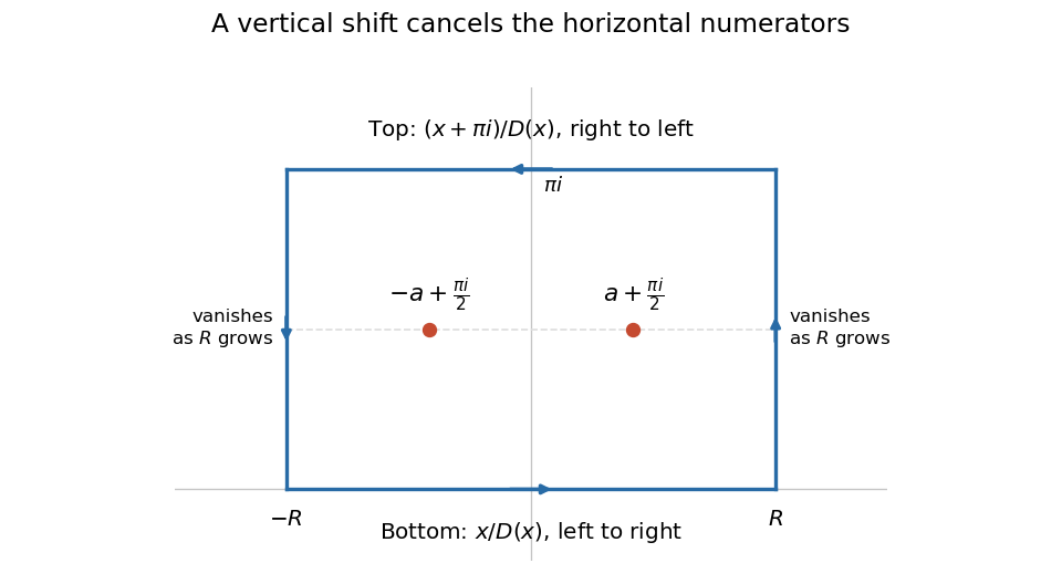
The choice of numerator $z$ makes the horizontal sides useful. The hyperbolic sine satisfies $\sinh (z+\pi i)=-\sinh z$, so $D(x+\pi i)=D(x)$. Consequently the lower and upper contour integrals, with their actual orientations, add toIt remains to justify discarding both vertical sides. On either side $z=\pm R+iy$, $0\le y\le \pi$, the reverse triangle inequality and part (b)(ii) implyThis lower bound is positive for sufficiently large $R$. Also $|z|\le R+\pi$ and each vertical side has length $\pi$. The estimation lemma bounds the absolute value of the sum $V_R$ of the vertical contributions byThe real improper integral converges absolutely, since its integrand is continuous on the real axis and decays like $4e^{-2|x|}$ at infinity. Combining all four sides and taking $R\to \infty$ givesThereforeAn independent real-variable check uses the hyperbolic tangent substitution $u=\tanh x$: the integral becomes ${\int }_{-1}^{1}du/({\cosh }^{2}a-u^2{\sinh }^{2}a)$. Its antiderivative uses the inverse hyperbolic tangent, giving $2\mathrm{arctanh}(\tanh a)/(\sinh a\cosh a)=4a/\sinh (2a)$. As $a\downarrow 0$, this tends to $2$, agreeing with ${\int }_{-\infty }^{\infty }{\mathrm{sech}}^{2}xdx=2$ and checking the factor of two.

Assume positive, counterclockwise orientation of a contour. Factor the polynomial denominator asOnly $z=\pm (\sqrt{3}-\sqrt{2})$ lie inside the unit circle. These are simple poles. Writing the denominator as $P(z)$, their residues areThe residue theorem therefore givesReversing orientation of a contour changes the sign.

The winding number records how many net turns a closed piecewise smooth curve makes around a chosen point $w$. Counterclockwise turns contribute positively, clockwise turns negatively. It measures a traversal, including repeated visits; a drawing of the curve's outline alone can lose that information. For a closed curve $\gamma$ avoiding $w$,Equivalently, continuously follow an argument of $\gamma (t)-w$ along one journey and divide its total change by $2\pi$. The start and endpoint agree as complex numbers, so the change is an integer number of full turns. The principal argument at the endpoints cannot retain those turns; a continuous choice along the parametrized path can.^[ref]

For $\gamma (t)=e^{it}$, $0\le t\le 2\pi$, the winding number about zero is one. Traversing the same unit circle twice makes it two; reversing its orientation of a contour makes it negative. The winding number about $w=2$ is zero: the same journey now stays to one side of the point being measured. Joining one counterclockwise loop and one clockwise loop around zero gives net winding number zero even though both loops encircle zero.

The winding number does not change during a homotopy of closed curves avoiding $w$. This is why it is useful: complicated curves can often be deformed to simple ones whose count is obvious. The argument principle transfers that robust geometric integer to a count of zeros of a function and poles. The example in boundary sampling can miss winding shows why finite samples of a curve need control between samples before they can certify the same winding number.