The positive energy theorem concerns the total gravitational energy of isolated systems, rather than a pointwise gravitational energy density. Its standard asymptotically flat form isHere are the hypotheses used in a spinorial proof. Take smooth, complete, three-dimensional initial data in general relativity with a spin structure, no inner boundary, and finitely many asymptotically Euclidean ends. Assume the usual differentiable falloff , , , with sufficiently decaying further derivatives and integrable matter densities. The Hamiltonian constraint and momentum constraint must hold, and the matter must satisfy the dominant energy condition. These hypotheses exclude a naked singularity or an unaccounted boundary flux from the argument. An oriented three-manifold admits a spin structure; in higher dimensions the spinorial proof needs this as an additional assumption. Work in signature and units .
Let be the future unit normal, choose , and define and . With this convention the Hamiltonian constraint and momentum constraint readThe dominant energy condition implies . The asymptotic charges are the ADM energy and ADM momentum,These are boundary charges; a sign condition on alone does not visibly determine their sign.
Choose gamma matrices obeying , with spatial matrices Hermitian and anti-Hermitian. The relevant derivative is the Sen spinor connection, not just the intrinsic spin connection:The symmetric extrinsic curvature makes . This is an elliptic differential operator with the ordinary spatial Dirac operator as principal part. Solve the Witten spinor equation , with constant at the end under consideration and zero asymptotic constants at any other ends.
The central algebraic ingredient is the Witten-Nester identity. Define , the future-directed Dirac current , and the Nester two-formIn an orthonormal frame . Since is Hermitian with eigenvalues for any unit spatial vector , . Thus the Dirac current is future causal. Differentiate the Nester two-form by the product rule. The antisymmetric second-derivative terms reduce using the spinor curvature identityThe Clifford algebra and the first Bianchi identity turn the curvature contraction into the Einstein tensor. The spatial derivative terms give the difference of two squares. Projecting onto therefore givesThe constraints are exactly the normal components of the Einstein field equations needed here. Moreover,For a solution of the Witten spinor equation, both terms left in this divergence are nonnegative.
There is an essential analytic step: an asymptotically constant spinor field solving the Witten spinor equation must actually exist. Extend the chosen constant smoothly from infinity to a field . Then is square-integrable. For compactly supported fields , the same Witten-Nester identity has zero boundary flux and givesThe asymptotically Euclidean Hardy inequality in Euclidean space, local elliptic estimates and this identity supply the coercive estimate in the weighted first-order Sobolev space of decaying corrections. One way to see why a compact-region error cannot spoil coercivity is to assume the estimate fails and take a normalized sequence whose Dirac operator tends to zero. Local compactness and the estimate on the ends produce a decaying homogeneous solution. Integrating the identity with cutoffs shows that such a solution is parallel for the Sen spinor connection. A parallel field tending to zero at infinity is zero, contradicting its normalization. The end estimates exclude escape of the normalized sequence to infinity.
More constructively, on this completed correction space solvefor every compactly supported , using the Lax-Milgram theorem. Set . Since is formally skew-adjoint in the positive spatial spinor inner product, the residual is a square-integrable weak solution of . Elliptic regularity makes it smooth. Cutoff integration of the identity excludes a nonzero square-integrable homogeneous solution: it would be parallel, whereas a nonzero parallel field has nonzero limiting norm on an asymptotically Euclidean end and cannot be square-integrable. Hence . Weighted elliptic estimates then give the required asymptotic decay of . This supplies elliptic existence of a Witten spinor, rather than assuming it from the sign of a formal integral.
Finally integrate the Witten-Nester identity over . The ADM boundary term of the Nester two-form isTo identify this boundary term, expand the asymptotic spin connection to first order in . Its flux is half of ; the extrinsic curvature contribution is . Their coefficients give precisely the two charges displayed above. The derivative of the decaying spinor correction has zero leading integrated flux by antisymmetry, and the higher-order terms vanish with the falloff. ThusChoose a normalized asymptotic spinor field that is an eigenvector with eigenvalue of . Then and . Choosing proves ; if , any such choice gives . This is positivity in every asymptotic frame, not only the zero-momentum case.
The zero-energy rigidity also follows from the vanishing integrals. If , then and the construction for a basis of asymptotic spinors produces a basis of parallel fields. Their spinor curvature identity forces the spatially pulled-back spacetime curvature to vanish; the nonnegative matter terms vanish too. The resulting Gauss–Codazzi equations are those of a hypersurface in Minkowski spacetime, and its vacuum development is flat. Completeness and the ordinary Euclidean asymptotic end rule out a nontrivial flat quotient. The initial hypersurface need not have : a curved spacelike slice of Minkowski spacetime also has zero ADM energy. The proof works by converting an asymptotic energy charge into a nonnegative bulk integral, with the spinor equation and its existence supplying the crucial bridge.
Use units and put . The static patch of de Sitter spacetime has radial factor . A Wick rotation makes its radial-time metric positive:Near the cosmological horizon, write . Then andin the radial-time directions. Thus must be an angle of period . A larger integer multiple would give a conical excess rather than a smooth origin. The Euclidean black-hole regularity condition givesThis de Sitter horizon temperature uses the time normalization at , where is proper time; static observers at other radii see the corresponding Tolman temperature law redshift.
Vary the gravitational Euclidean action with respect to . The identities and the integrated variation of the scalar curvature yield, after discarding the assumed boundary term,The resulting vacuum Einstein field equations are thereforeTracing in four dimensions gives , and substitution gives .
The smooth Euclidean geometry is compact. Explicitly, in Euclidean five-space useThese obey and induce precisely the above metric, so with the identified Euclidean time covers a round four-sphere once. Neither the collapsing two-sphere at nor the collapsing time circle at is a physical boundary. Since , its volume and on-shell Euclidean action areThe semiclassical partition function is , and follows from the free energy relation . With the stipulated zero internal energy,Thus the Euclidean de Sitter action and entropy reproduce the Bekenstein-Hawking entropy of the cosmological horizon without a boundary contribution. Restoring constants, .
Take and write . Integrating gives the Schwarzschild tortoise coordinateThe advanced and retarded Eddington-Finkelstein coordinates are respectively and . Substituting or givesBoth radial-time blocks have determinant and smooth coefficients at . Consequently the Schwarzschild event horizon is a coordinate singularity of the original chart, not a degeneracy of the geometry. The Kretschmann scalar is finite there, while it diverges at . Angular coordinate degeneracies at the polar axes are removed separately by ordinary sphere charts.
The ingoing Eddington-Finkelstein coordinates extend the right exterior through its future black hole horizon. Radial null geodesics obey either or . Inside , the latter also moves towards smaller as increases, and the future-directed ingoing family has decreasing . Thus neither family can escape to the exterior. The future horizon is the boundary separating points that can send signals to future null infinity from those that cannot. The retarded chart extends through the past horizon instead. Reversing the time orientation gives the white hole: future-directed signals can leave it, but exterior signals cannot enter it. These are distinct branches in the eternal extension; the white-hole branch need not occur in a spacetime formed by collapse.
For a simultaneous extension through both branches, start in the right exterior and define the Kruskal–Szekeres coordinatesTheir product and the extended metric areIndeed and transform into the displayed expression. The function of on the right of the product relation has derivative , nonzero at , so is a smooth function of across zero. The coefficient of there is , finite and nonzero. Allowing either sign of therefore gives the regular maximal extension with and .
With and , the radial metric is a positive multiple of . The two exterior regions have and . The future interior, or black hole region, has ; the past interior, or white hole region, has . The Killing horizons are and , meeting on the bifurcation surface at .
For the Penrose diagram, compactify the null variables before forming time and space:This Schwarzschild conformal compactification preserves radial null directions because . The ranges bound the diagram, and cuts off its future and past tips. On with , , so the future curvature singularity is . The past curvature singularity is similarly . Both have and are spacelike. The horizon lines remain .
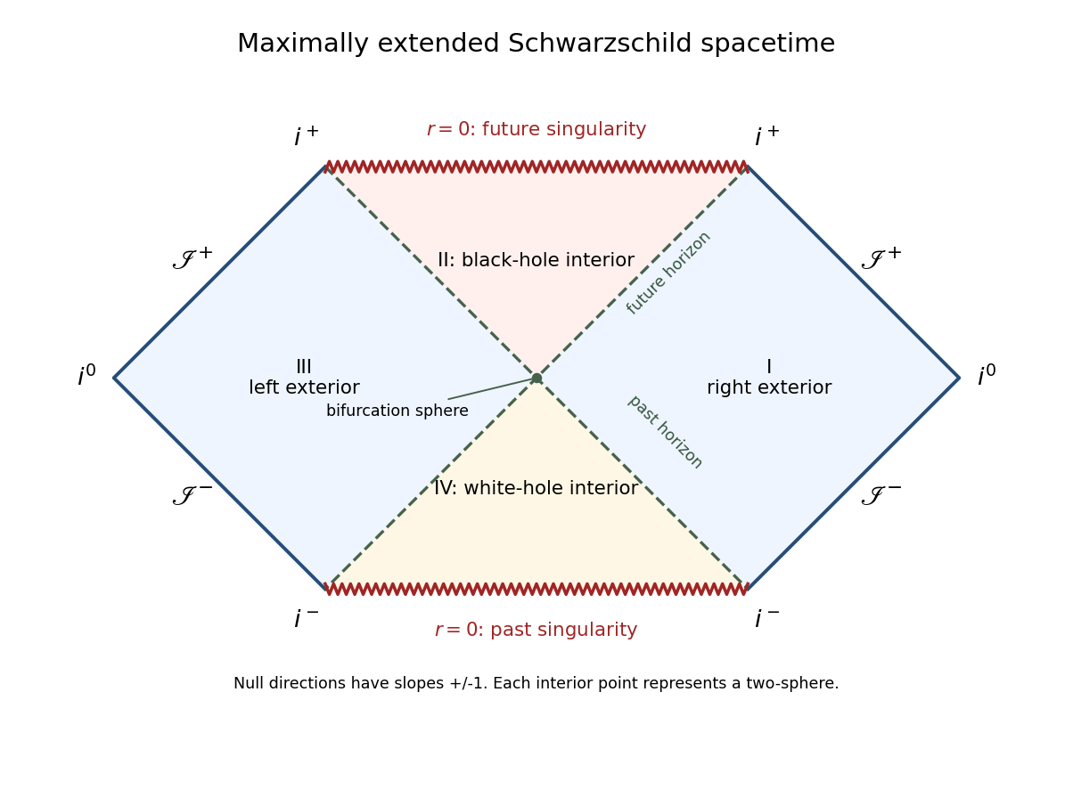
Penrose diagram of maximally extended Schwarzschild spacetime, with two exteriors, black and white hole interiors, horizons and conformal infinities
. Details. 
Each point of this radial Penrose diagram represents a two-sphere, except at limiting boundaries. Each exterior has its own future and past null infinity, and . For example in the right exterior, at fixed gives , whereas at fixed gives . Its spacelike infinity is ; its future and past timelike infinity are the vertices and . The left exterior has the reflected counterparts. These conformal boundary points are ideal endpoints, not finite-distance spacetime events; the physical affine or proper parameters of escaping geodesics diverge.
The horizons are regular null surfaces, while the horizontal boundaries are genuine curvature singularities. The central point represents the regular bifurcation surface, not a singularity. Future-directed radial causal curves have nondecreasing , so a curve cannot go from one exterior to the other: changing the requisite signs would require one null variable to decrease. Crossing a future horizon instead leads towards the future singularity. The maximal extension has two causally disconnected exteriors, a future black-hole region and a past white-hole region.
Let . A positive-radius horizon requires a root of , givingFor the usual asymptotically flat Reissner-Nordstrom spacetime, the black-hole conditions areThe strict inequality gives a nonextremal outer event horizon at ; equality gives an extremal black hole. If with , there is no horizon and the central curvature singularity is naked. Nonpositive cannot supply a positive-radius black-hole horizon; is Minkowski spacetime. For , the zero root is the singularity, not an additional regular horizon.
In the static coordinates the vector has constant components and every metric component is independent of . Its Lie derivative therefore satisfiesFor the torsion-free Levi-Civita connection, , proving the Killing equation directly. This also normalizes the Killing vector field to unit time translation at infinity.
At , . Use the regular advanced chart with , in whichOn the horizon, . Thus the Killing vector field is both null and normal to the horizon, and its orbits generate that Killing horizon. The normal lines of a null hypersurface are null geodesics, possibly with nonaffine parameter. To see this without assuming a separate geodesic property, the Killing equation givesRestriction to the future horizon therefore givesThe acceleration is proportional to the tangent, which is exactly the geodesic equation with a nonaffine parameter. An affinely parametrized tangent can be obtained by rescaling along each generator; that rescaled vector need not itself extend to a spacetime Killing vector field. At a nonextremal bifurcation surface, vanishes, so a nonzero generator tangent must be described in a regular affine parametrization there.
On the past branch, use the retarded chart with radial-time cross term . Now at the horizon, so the same calculation yields the opposite signed nonaffinity. Since is constant and the spacetime is spherically symmetric, is constant over the future horizon. This gives the two signs in the horizon relation without assuming their value beforehand.
Factor . Its derivative at the outer horizon gives the Reissner-Nordstrom horizon surface gravityIt is positive for , and at reduces to the Schwarzschild surface gravity . For , the root is double and . Thus the horizon remains present when its surface gravity vanishes: it is a degenerate Killing horizon, and itself has affine parametrization along its nonzero horizon generators. The strictly positive-constant description applies only to the nonextremal case; the zero value is the legitimate extremal limit.
Articles by others on the same topic
There are currently no matching articles.