The inequality in the printed rule is reversed. With the stated definition of , a larger score favors group one. For example, in one dimension take , , , equal priors and . The score is , and , whereas the printed rule assigns group two. The correct Bayes classifier follows from minimizing the error cost as follows.
Let be the region assigned to group one, let be its multivariate normal density, and let each misclassification cost , with zero cost for correct classification. The expected cost isThe permitted integral-minimization result therefore selects . Points of equality may be assigned to either group without changing the risk. Equivalently, the Bayes classifier chooses the larger posterior probability.
For positive priors and a common positive-definite covariance matrix, the normalization constants cancel in the likelihood ratio. Expanding the two quadratic forms givesThus the correct Gaussian Bayes classifier, choosing group one on ties, isThis proves the intended classification result with the necessary correction. Equal error costs remove from the decision, while prior odds determine the threshold.
Use a multivariate normal distribution within each species, a common positive-definite covariance matrix, equal prior odds and equal misclassification costs. Assume the training observations are independent and representative of the populations. Substituting the sample means and pooled sample covariance matrix gives a fitted linear discriminant analysis rule, rather than a rule with known population parameters.
The determinant of the pooled covariance is , soThe midpoint of the sample means is , whose scalar product with is . Hence the fitted log likelihood ratio isAssign fattus when and apathus when ; either assignment is optimal on under equal priors. The separating line is , with fattus below it. As a sign check, the scores at the two sample means are and , respectively. This uses the corrected Gaussian Bayes classifier from (a).
Evaluating the fitted linear discriminant analysis score givesThe fifth individual lies exactly on the discriminant boundary. Its two fitted posterior probabilities are equal, so the equal-prior Bayes classifier cannot prefer either species. A specified tie convention could assign it to one species, but such an assignment would not be evidence favoring that species.
In the sketch the solid line is the equal-prior boundary. The dashed line is the prior-dependent Gaussian discriminant boundary for the altered priors in (iii).
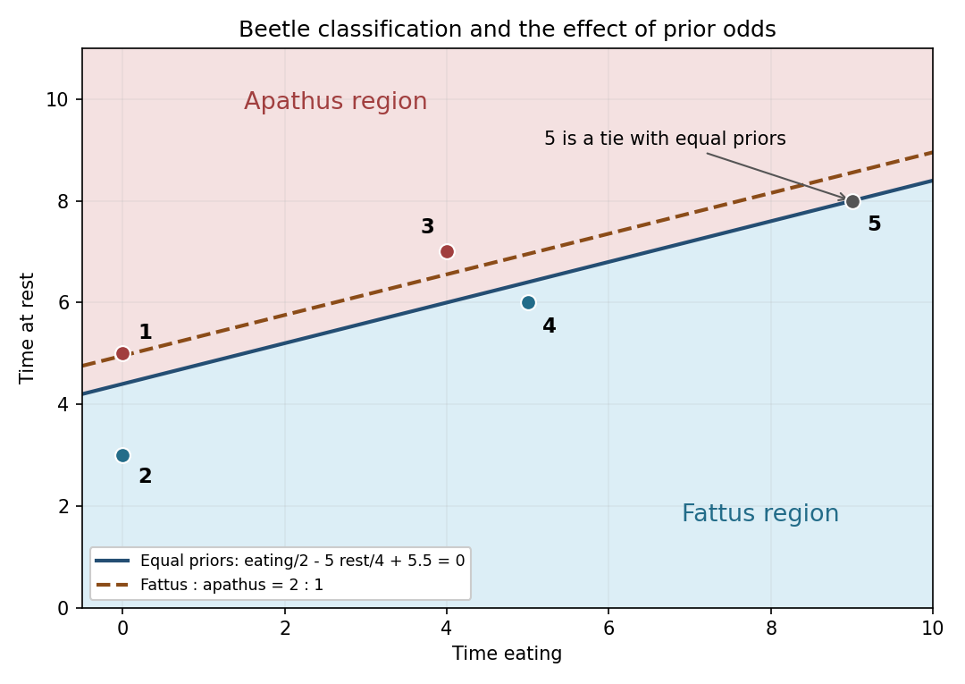
Beetle classifications and the parallel boundary shift when fattus has twice the prior probability
. Details. 
Now the prior odds are . The fitted log posterior odds are , so the Gaussian Bayes classifier assigns fattus when . The prior-dependent Gaussian discriminant boundary becomesIt moves upwards parallel to the original line by , expanding the fattus region. This is the dashed line in the sketch. The fifth individual's fitted log likelihood ratio remains zero, but its posterior odds become , giving posterior fattus probability .
The fifth individual is now classified as fattus. For completeness, the other four classifications remain apathus, fattus, apathus and fattus: their scores lie on the same side of the new threshold as before.
Articles by others on the same topic
There are currently no matching articles.