Let . Independence of the standard normal distributions gives , , and joint densityChoose a matrix with , for example the lower-triangular factor from the Cholesky decomposition. It exists and is nonsingular because is a symmetric positive-definite matrix. Then the required simulation isIt has mean and covariance matrix , and every linear combination of its coordinates is Gaussian, so it has the required multivariate normal distribution.
For the multivariate normal density, apply the change of variables formula to . Its absolute Jacobian determinant is , andHenceThe nonsingularity assumption is needed for a density with respect to -dimensional Lebesgue measure.
Take the coordinate-selection matrixThen , and . The permitted result on a linear image of a multivariate normal vector therefore givesThis is the marginal distribution obtained by discarding the other coordinates. The conclusion holds also for a positive-semidefinite marginal covariance: in that case the Gaussian law may be degenerate and need not have a full-dimensional density. If the original covariance is positive definite, its principal block is positive definite as well.
Assume an independent Gaussian sample, positive-definite population covariance, and . Define the sample mean and unbiased sample covariance matrix byThe standard test is based on Hotelling's T-squared statisticReject the null hypothesis for large values. Under the null its exact distribution isThe factor uses the unbiased, divisor- covariance convention. Normal-sample theory makes independent of the residual covariance, whose whitened version has a Wishart distribution; this yields the stated F-distribution. The condition gives invertibility of almost surely and positive denominator degrees of freedom.
This is also the likelihood-ratio test. To see the connection, put and . The maximized covariance estimates under the unrestricted and null models are and , respectively. The determinant identity for a rank-one update givesThus the likelihood ratio is , decreasing in . The term best is understood here as this standard likelihood-ratio, affine-invariant procedure; a two-sided multidimensional alternative does not specify a single direction to optimize power against.
For the transformed sample , with the prescribed nonsingular coordinate transformation, we haveConsequentlyThis proves the affine invariance of Hotelling's statistic. The statistic, its p-value and its test decision are unchanged by a nonsingular affine transformation, provided the null mean is transformed with the data. Changes of units and rotations are included.
The inequality in the printed rule is reversed. With the stated definition of , a larger score favors group one. For example, in one dimension take , , , equal priors and . The score is , and , whereas the printed rule assigns group two. The correct Bayes classifier follows from minimizing the error cost as follows.
Let be the region assigned to group one, let be its multivariate normal density, and let each misclassification cost , with zero cost for correct classification. The expected cost isThe permitted integral-minimization result therefore selects . Points of equality may be assigned to either group without changing the risk. Equivalently, the Bayes classifier chooses the larger posterior probability.
For positive priors and a common positive-definite covariance matrix, the normalization constants cancel in the likelihood ratio. Expanding the two quadratic forms givesThus the correct Gaussian Bayes classifier, choosing group one on ties, isThis proves the intended classification result with the necessary correction. Equal error costs remove from the decision, while prior odds determine the threshold.
Use a multivariate normal distribution within each species, a common positive-definite covariance matrix, equal prior odds and equal misclassification costs. Assume the training observations are independent and representative of the populations. Substituting the sample means and pooled sample covariance matrix gives a fitted linear discriminant analysis rule, rather than a rule with known population parameters.
The determinant of the pooled covariance is , soThe midpoint of the sample means is , whose scalar product with is . Hence the fitted log likelihood ratio isAssign fattus when and apathus when ; either assignment is optimal on under equal priors. The separating line is , with fattus below it. As a sign check, the scores at the two sample means are and , respectively. This uses the corrected Gaussian Bayes classifier from (a).
Evaluating the fitted linear discriminant analysis score givesThe fifth individual lies exactly on the discriminant boundary. Its two fitted posterior probabilities are equal, so the equal-prior Bayes classifier cannot prefer either species. A specified tie convention could assign it to one species, but such an assignment would not be evidence favoring that species.
In the sketch the solid line is the equal-prior boundary. The dashed line is the prior-dependent Gaussian discriminant boundary for the altered priors in (iii).
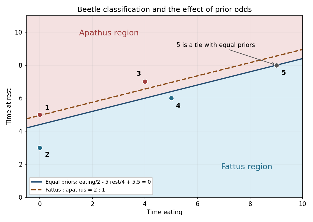
Beetle classifications and the parallel boundary shift when fattus has twice the prior probability
. Details. 
Now the prior odds are . The fitted log posterior odds are , so the Gaussian Bayes classifier assigns fattus when . The prior-dependent Gaussian discriminant boundary becomesIt moves upwards parallel to the original line by , expanding the fattus region. This is the dashed line in the sketch. The fifth individual's fitted log likelihood ratio remains zero, but its posterior odds become , giving posterior fattus probability .
The fifth individual is now classified as fattus. For completeness, the other four classifications remain apathus, fattus, apathus and fattus: their scores lie on the same side of the new threshold as before.
Principal component analysis replaces the original coordinates by orthogonal linear combinations, ordered so that the first few retain as much variance as possible. It gives a lower-dimensional summary for visualization or compression and reveals the main directions of variation. A direction of large variance need not be the direction most useful for classification.
Write . For a unit vector , the centered score has varianceMaximizing this Rayleigh quotient with a Lagrange multiplier givesThus a maximizing direction must be an eigenvector of the covariance matrix. To identify the maximum, use the spectral theorem for real symmetric matrices to choose an orthonormal basis of eigenvectors , with eigenvalues . Writing givesEquality is attained at . Consequently the first population principal component isFor each subsequent principal component, maximize the same variance over unit coefficient vectors orthogonal to all the previously chosen ones. Restricting the expansion above to the remaining eigenvectors gives , then , and so on. ThusThe principal components are uncorrelated; they need not be independent unless additional distributional assumptions, such as joint Gaussianity, hold. Their total variance is . Signs of eigenvectors are arbitrary, and a repeated eigenvalue permits any orthonormal basis in its eigenspace. In sample principal component calculations, replace by the sample mean and by the sample covariance matrix.
For , direct multiplication by the sample covariance matrix givesIt is therefore an eigenvector, with eigenvalue . Normalization gives , so the corresponding sample principal component isIts coefficients are proportional to the required vector. The remaining eigenvalues calculated in (ii) are smaller, confirming that this is the first principal component.
Let be the three supplied coefficient vectors, in their displayed order. Multiplication by the sample covariance matrix givesThe four vectors are pairwise orthogonal, with norms , , and . Hence form an orthonormal basis of eigenvectors. The variance of the principal component with unit coefficient vector is its eigenvalue . Using unnormalized coefficient vectors would instead give variances and would not produce the desired proportions.
The total variance isTherefore the explained variance of a principal component isThe first two principal components together account for , and the first three account for of the total variance.
The first principal component has equal positive coefficients on the three academic subjects and zero coefficient on physical education. It measures overall academic performance in those subjects and explains of the variance. The large positive academic covariances explain why these subjects vary predominantly together.
The second principal component has normalized coefficients approximately . It is mainly a physical-education score, with a small adjustment for the physics-versus-mathematics contrast, and explains of the variance. The small physical-education covariances with the academic subjects make this direction close to a separate physical-education axis. This is an interpretation of the observed covariance matrix, not proof of distinct causal abilities or statistical independence.
The third principal component compares physics and mathematics together against biology: its coefficient vector is . It captures subject balance rather than overall academic performance, accounting for of the variance. The fourth principal component primarily contrasts physics with mathematics, with a smaller physical-education correction; its normalized coefficients are approximately , and it accounts for the remaining . Changing all signs in any component reverses its score without changing the interpretation of its contrast or its explained variance of a principal component.
A two-component summary separates broad academic performance from predominantly physical-education performance and retains about of the variation. It still discards about , including differences between academic subjects. Whether that loss is acceptable depends on the purpose: an overall summary may use two principal components, whereas studying subject-specific strengths requires the later principal components too. A single principal component would lose most of the physical-education information.
If the change is purely a rescaling of the physics mark, write , where . The sample covariance matrix transforms asThe physics variance is multiplied by , becoming approximately . Each covariance between physics and another subject is multiplied by , and all other entries stay unchanged. Principal component analysis on this new sample covariance matrix maximizes variance in the new numerical units, so its eigenvectors and explained variance of a principal component generally change. Physics receives disproportionately greater influence simply because its unit has changed.
One solution is to convert the physics marks back to the original scale before doing principal component analysis. Alternatively, use principal component analysis on a correlation matrix: standardize every subject byA positive change of units multiplies both a centered variable and its standard deviation by the same factor. Thus it leaves and the sample correlation matrix unchanged.
Correlation-based principal component analysis is invariant under positive changes of units; covariance-based principal component analysis is not. Standardizing gives each subject unit variance, which is a different weighting choice and can emphasize relatively low-variance subjects. If the revised assessment changes the scores themselves rather than just their units, its sample correlation matrix may also change, and mere standardization cannot recover the original analysis.
Write for two rows of the data matrix and . Three possible dissimilarities for continuous variables are the following.
The Euclidean distance isIt is simple and has the usual geometric interpretation when coordinates have comparable units. Its disadvantage is sensitivity to the numerical scales: a change of units or a high-variance variable can dominate it. Strongly correlated coordinates can also give repeated weight to essentially the same information. Squared Euclidean distance is useful in some methods, but is not itself a metric because it need not satisfy the triangle inequality.
The standardized Euclidean distance iswhere is the sample variance of coordinate across individuals. It measures differences in standard-deviation units and is invariant under positive coordinate rescalings when the scales are estimated consistently. It is useful for differently measured variables, but requires nonzero sample variances, ignores correlations between coordinates and can give excessive influence to a low-variance noisy variable. With fixed positive scales it is a Euclidean distance after a diagonal change of coordinates, so it is a metric.
The Mahalanobis distance iswhere is the pooled sample covariance matrix of all individuals. If is its Cholesky decomposition, then : it is Euclidean distance in whitened coordinates. It adjusts for both scales and correlations, avoiding duplicate weight for highly correlated variables, and is invariant under nonsingular affine transformations when the sample covariance matrix is transformed accordingly. No multivariate normal distribution assumption is required merely to define the distance. However, must be a positive-definite matrix; when there are too few observations or dependent coordinates, its inverse is unavailable. Estimation of can also be unstable and sensitive to outliers. These trade-offs determine whether covariance adjustment is preferable to the simpler distances.
A metric dissimilarity must satisfy nonnegativity, separation, symmetry and the triangle inequality:The underlying objects must be specified: here they are binary measurement profiles, rather than labels attached to individuals.
Let count coordinate pairs of the indicated types. The simple matching coefficient is , so its complementary dissimilarity is . Counting mismatches in every pair gives the dissimilarity matrixFor the Jaccard coefficient, joint absences are excluded: . Thus the Jaccard distance is , givingOnly the pair of individuals two and four has a joint absence. Their profiles have one shared presence, two mismatched presences and one joint absence, giving dissimilarities and , respectively. All other pairs have a presence in at least one profile at every coordinate, so the two denominators coincide.
For the requested metric property of simple matching dissimilarity, write a general pair of -coordinate binary profiles as . Thenwhich is the normalized Hamming distance. It is nonnegative and symmetric, and equals zero exactly when all coordinates match. For each coordinate, a mismatch between and forces a mismatch between or between . ThereforeSumming and dividing by proves the triangle inequality, establishing all four metric properties. Simple matching dissimilarity is a metric on binary profiles. If two separately labelled individuals have identical profiles, it gives zero distance between them, so on those labels it is only a pseudometric. The four profiles here are distinct, so this distinction does not prevent from defining a metric on the given sample.
There is a defect in the stated geometric interpretation of the data. The supplied numbers cannot be Euclidean distances, becauseThey violate the triangle inequality; independently, . Nevertheless, both clustering algorithms are defined for this symmetric dissimilarity matrix. The calculations below retain the supplied numbers and use agglomerative clustering of nonmetric dissimilarities, rather than silently inventing Euclidean replacement data.
In single-linkage clustering, the intercluster dissimilarity isThe closest pair is , merging at . Among the remaining clusters the next closest pair is , merging at . The three intercluster dissimilarities are nowConsequently merges with at , using the cross-pair . The remaining point joins at , using . The dendrogram thus hasThe close pairs and are the clearest early groupings. A cut between and produces these two pairs and the singleton ; a cut between and produces and . Single-linkage clustering builds chains through close cross-pairs, so the merge at does not mean every pair in is that close: . The data alone do not prescribe a unique number of clusters.
For complete-linkage clustering, replace the minimum by the maximum:The first two merges remain at and at . SubsequentlyThus joins at . The final maximum between and is , givingBoth the topology and the later heights of the dendrogram change: complete-linkage clustering attaches to before joining that group to , rather than merging the two pairs first. Its control of the largest within-cluster separation makes it less susceptible to the chaining seen with single-linkage clustering.
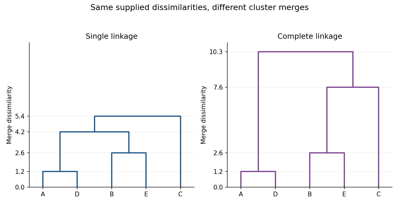
Single-linkage and complete-linkage dendrograms for the supplied five-subject dissimilarities
. Details. 
Articles by others on the same topic
There are currently no matching articles.