Let denote one-component velocity variance, the longitudinal velocity correlation, and the signed longitudinal structure functions. Homogeneity gives , while the third-order convention here is . Thus the Kármán-Howarth equation becomesThe mean kinetic energy per unit mass is , so its decay gives . In the universal equilibrium range, the small-scale variation is negligible at leading order, hence . Integrating from zero and using regularity givesThe Kolmogorov equation for structure functions is thereforeFor finite local unsteadiness the right side has the additional term ; dropping it is the local-equilibrium approximation used here.
In the inertial range the viscous term is also negligible, leaving the Kolmogorov four-fifths law, . Its coefficient and sign follow from the exact energy balance and Kármán-Howarth equation, rather than from dimensional similarity. It supplies a firm third-order constraint on Kolmogorov 1941 theory and measures the forward energy cascade, while leaving the second- and higher-order exponents open to internal intermittency corrections.
Put , and , where . The small- Taylor series giveIn the Kármán-Howarth equation, the coefficient of on the left is . On the right, the triple-correlation term contributes and the viscous term contributes . HenceComparing with the mean enstrophy balance identifies the mean vortex stretching:Also , whereas differentiability gives . Thus . Homogeneity makes , so the longitudinal velocity-gradient skewness is . Substitution givesPositive mean vortex stretching therefore requires negative skewness. A centered Gaussian distribution has zero third moment, so the derivative statistics cannot be Gaussian. This conclusion uses the physically positive mean stretching, not homogeneity alone.
The probability density function has mean zero but a longer or stronger negative tail, representing intermittent compression. The illustration uses a standardized Gaussian mixture distribution solely to sketch this sign of skewness; it is not turbulence simulation data or a fitted universal distribution.
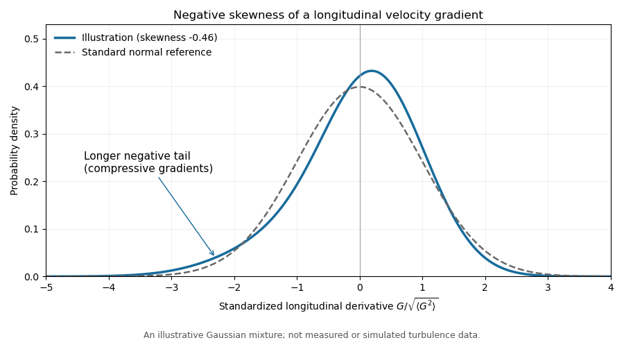
Illustrative negatively skewed longitudinal velocity-gradient density
. Details. 
Combining the Kolmogorov two-thirds law with the Kolmogorov four-fifths law gives the velocity increment skewness in the inertial range:The constant-skewness turbulence closure assumes this same value throughout the universal equilibrium range, including the dissipative crossover. This is an extra modeling assumption; neither similarity law establishes it near .
Write , , and . Since and , substituting into the Kolmogorov equation for structure functions givesDividing by yields the normalized constant-skewness structure-function equation:At small , , recovering for differentiable velocity increments. At large , the dominant balance gives , recovering the assumed Kolmogorov two-thirds law.
This turbulence closure is inexpensive: a single ordinary differential equation interpolates between the two regimes while respecting the local third-order balance. Its prescribed skewness cannot independently predict scale-dependent derivative statistics, transient spectral evolution or internal intermittency.
EDQNM closure instead evolves the turbulent energy spectrum through modeled spectral triad interactions. Its quasi-normal fourth-order approximation is supplemented by eddy damping and a Markovian treatment of correlation memory. It retains more information about scale-dependent transfer and evolving spectra, at the cost of spectral integrals and modeled damping times. It is still approximate and does not automatically describe coherent structures or internal intermittency. The simple constant-skewness model is therefore useful as an equilibrium interpolation; EDQNM closure addresses a broader spectral evolution problem.
Articles by others on the same topic
There are currently no matching articles.