At order , scalar particle–antiparticle scattering has a -channel photon exchange and an -channel annihilation and recreation diagram. They are shown below, with incoming momenta and outgoing momenta . The seagull vertex has only two scalar legs and does not yield a four-scalar tree diagram at this order.
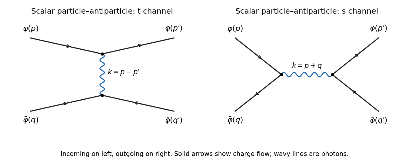
Leading scalar particle–antiparticle scattering diagrams with exchanged and annihilation-channel photons
. Details. 
For the exchange graph, let . Apart from overall charge signs, the two scalar currents are and . The external mass shell conditions giveFor the annihilation graph, , with currents and , again up to vertex signs. Their contractions are and . Thus each graph couples the photon to conserved currents, the relevant scalar quantum electrodynamics Ward identity.
Write and . conserved current means and . For , contraction with the Coulomb-gauge photon propagator gives, displaying the rational identity before the pole boundary limit,We used . Restoring the common Feynman i-epsilon prescription yields the Coulomb-gauge propagator between conserved currents resultHence each on-shell tree amplitude can use the Lorentz-invariant propagator. This is equality after contraction, not equality of the gauge-dependent tensors. At , the separate Coulomb-gauge terms are ill-defined; combine them first and take the conserved-current limit. The combined expression has only the physical photon pole.
Articles by others on the same topic
There are currently no matching articles.