Use the same Minkowski metric as in Question 1. For the conjugate charged field, the kinetic term means , with . Thus the conjugate field has the opposite charge in the gauge covariant derivative.
For any real smooth function , make the local transformationThe electromagnetic field tensor is unchanged because the mixed derivatives of commute. Directly,Its conjugate transforms with the inverse phase, so is invariant. The mass term depends only on and is invariant as well. All terms of the action are therefore unchanged. This proves the local U(1) gauge symmetry of scalar electrodynamics.
A gauge redundancy relates different field representatives of the same physical configuration. For example, the transformation just exhibited changes and the scalar phase but leaves , and all other gauge-invariant operators unchanged. Fixing a gauge removes this freedom; it does not remove a physical symmetry-related state. In canonical quantization, local transformations trivial at the boundary are generated by the Gauss law constraint in gauge theory, and physical states satisfy that constraint.
A global symmetry in field theory instead has a spacetime-independent parameter and can act nontrivially on physical states. For a continuous global symmetry in field theory, Noether theorem gives a conserved charge that generates the transformation and labels the states; discrete global symmetries do not acquire a Noether current from the same infinitesimal theorem. These are statements about physical transformations, rather than merely whether a parameter is written as a constant or a function.
Boundary conditions matter in gauge theory. gauge transformations that vanish at spatial infinity are redundancies, while transformations nontrivial at infinity may act through a physical electric charge. In particular a constant phase transformation can survive as a global charge symmetry rather than being quotiented out with the local gauge redundancy. Thus local gauge redundancy is a redundancy of description; genuine global symmetry in field theory can distinguish physical states and charges, with the boundary qualification made explicit.
Expand the gauge covariant derivative in the scalar kinetic term:The cubic interaction is thereforeFor an incoming scalar momentum and outgoing momentum , derivatives give on the incoming field and on its outgoing conjugate. Multiplication by the factor from the interaction action gives the scalar electrodynamics three-point vertex .
The other vertex comes fromDifferentiating twice with respect to the identical photon fields gives a factor of two, so the seagull vertex is . There is no additional factor of two from the scalar fields, since the complex scalar field and its conjugate are distinct legs.
At order , scalar particle–antiparticle scattering has a -channel photon exchange and an -channel annihilation and recreation diagram. They are shown below, with incoming momenta and outgoing momenta . The seagull vertex has only two scalar legs and does not yield a four-scalar tree diagram at this order.
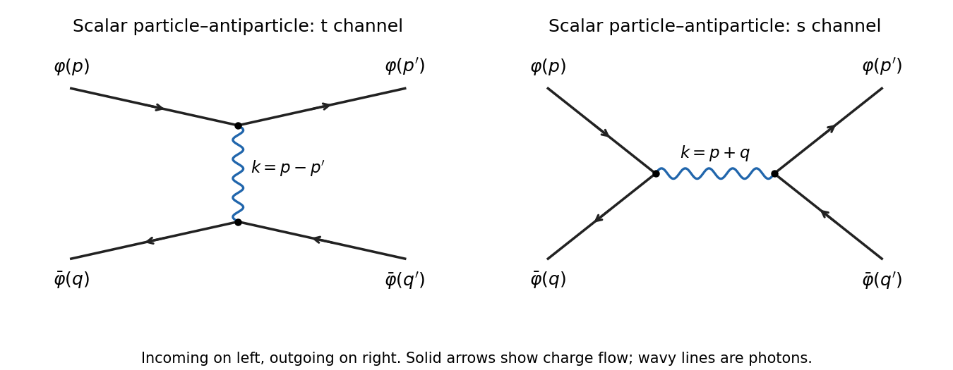
Leading scalar particle–antiparticle scattering diagrams with exchanged and annihilation-channel photons
. Details. 
For the exchange graph, let . Apart from overall charge signs, the two scalar currents are and . The external mass shell conditions giveFor the annihilation graph, , with currents and , again up to vertex signs. Their contractions are and . Thus each graph couples the photon to conserved currents, the relevant scalar quantum electrodynamics Ward identity.
Write and . conserved current means and . For , contraction with the Coulomb-gauge photon propagator gives, displaying the rational identity before the pole boundary limit,We used . Restoring the common Feynman i-epsilon prescription yields the Coulomb-gauge propagator between conserved currents resultHence each on-shell tree amplitude can use the Lorentz-invariant propagator. This is equality after contraction, not equality of the gauge-dependent tensors. At , the separate Coulomb-gauge terms are ill-defined; combine them first and take the conserved-current limit. The combined expression has only the physical photon pole.
Articles by others on the same topic
There are currently no matching articles.