The Pauli matrix multiplication law is , so . Block multiplication of the chiral gamma-matrix representation givesandThus the mixed anticommutators vanish and the spatial ones are . With the Minkowski metric convention ,These matrices therefore represent the required Clifford algebra.
Apply to the Dirac equation. Since partial derivatives commute, only the symmetric part of the gamma matrix product contributes:Here in the signature fixed above. The remaining operator is scalar in spinor indices, givingThis is the Klein-Gordon equation for each component, although the first-order Dirac equation additionally couples them.
For positive frequency take , with . Lowering the index in is important: putThese are commuting Hermitian matrices with . Their eigenvalues are , so they are positive definite for and positive semidefinite matrices for . Simultaneous diagonalization defines their positive square roots of a matrix and gives .
The plane-wave ansatz reduces the Dirac equation to , whereFor and , commutativity gives and . ThereforeThis is the Hermitian square-root construction of Dirac plane waves.
For negative frequency retain the future-directed momentum label and use . The equation is now . Its general solution iswith arbitrary two-spinor . The minus between its two blocks gives and . For these parametrizations span the two-dimensional positive- and negative-frequency solution spaces. At nonzero null momentum the square roots have complementary rank-one supports and still give the full two-dimensional kernels. If , both spinors have norm squared ; the positive one also has .
Both blocks of the given rotation matrix carry the same spin one-half representation, so a stationary spin-up state along the third axis uses the eigenspinor of . At rest , givingFor a massless particle moving along the positive third axis, with , andKeeping the same two-spinor label givesIt has positive helicity and positive chirality in the Weyl representation.
For spin-up along the first axis, take the normalized eigenspinor of , namely . At rest this givesFor momentum , using the square roots displayed in part (i) with the same label givesThis is the massless limit of a transverse canonical-spin label: it is the equal superposition of the negative-helicity left-chiral mode and the positive-helicity right-chiral mode. It solves the massless Dirac equation and has norm squared .
A qualification is essential if “spin along the first axis” is interpreted literally at zero mass. The fixed transverse rotation generator is , with , and the massless Hamiltonian at this momentum is . They anticommute. If and both held, then , whereas , forcing . Thus there is no nonzero positive-energy massless solution with that literal transverse-spin eigenvalue. The displayed nonzero spinor is the transported rest-spin label requested by the massive-to-massless construction, rather than a transverse-spin eigenstate.
The normalized Fock vacuum obeys for every momentum and . Taking adjoints gives . Of the four products in the mode expansion of , only has a nonzero vacuum expectation value. The commutator impliesConsequentlyThis unordered Wightman function differs from the time-ordered Feynman propagator when the temporal ordering is reversed.
Write and . By time ordering for a bosonic field,Reverse in the second integral. At fixed spatial momentum considerThe Feynman i-epsilon prescription places the poles at and . For , close in the lower half-plane, clockwise. The positive-energy residue and the orientation give . For , close counterclockwise in the upper half-plane; the negative pole has derivative denominator , and its residue gives . Thus , reproducing the time-ordered mode expression. We obtainThis is a distributional boundary value, not an absolutely convergent Fourier integral. As an independent normalization check, , so ; the numerator is with the question's definition of the propagator.
The Yukawa interaction has one real-scalar leg and an oriented fermion line at each vertex. At lowest connected order, two vertices exchange one scalar, so the diagrams are of order .
For two incoming fermions, there are two pairings of the outgoing fermions: the channel joins to and to , with scalar momentum ; the channel joins to and to , with scalar momentum . Fermion number conservation excludes an annihilation channel for two particles carrying the same charge.
For an incoming fermion and antiparticle, there is a -channel scalar exchange with momentum and an -channel annihilation and recreation diagram with momentum . Arrows on antiparticle lines run opposite to the direction of physical propagation. These are the four tree scattering in Yukawa theory diagrams shown below; all external momenta are labelled.
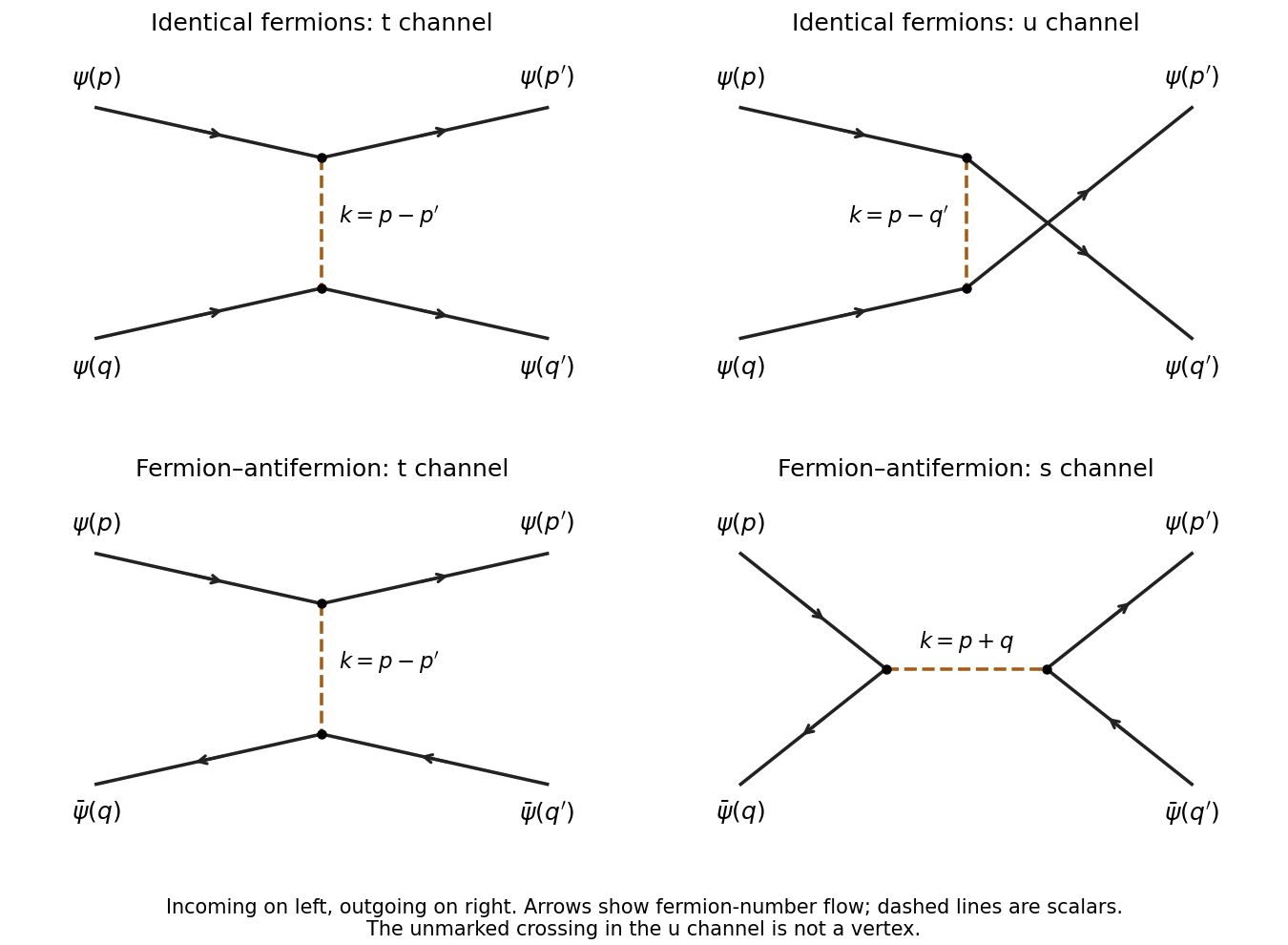
Tree-level scalar-exchange diagrams for fermion–fermion and fermion–antifermion scattering; incoming states on the left
. Details. 
The crossing in the -channel drawing is not a vertex. Dashed internal lines are the real scalar field; solid arrows show fermion-number flow.
Use the Feynman vertex for the scalar Yukawa coupling, the internal scalar propagator , incoming factors and outgoing Dirac adjoints . Define as the coefficient in the connected S-matrix element after removing its overall momentum-conserving Dirac delta function. A direct pairing contributesThe crossed pairing interchanges the identical outgoing fermions and therefore has a relative fermionic sign of minus. With and , the result isIt changes sign under exchange of the two outgoing momenta and spin labels, as required for identical fermions. No fermion spin sum or identical-particle phase-space factor belongs in this amplitude; those enter a relativistic scattering cross-section calculation.
Use the same Minkowski metric as in Question 1. For the conjugate charged field, the kinetic term means , with . Thus the conjugate field has the opposite charge in the gauge covariant derivative.
For any real smooth function , make the local transformationThe electromagnetic field tensor is unchanged because the mixed derivatives of commute. Directly,Its conjugate transforms with the inverse phase, so is invariant. The mass term depends only on and is invariant as well. All terms of the action are therefore unchanged. This proves the local U(1) gauge symmetry of scalar electrodynamics.
A gauge redundancy relates different field representatives of the same physical configuration. For example, the transformation just exhibited changes and the scalar phase but leaves , and all other gauge-invariant operators unchanged. Fixing a gauge removes this freedom; it does not remove a physical symmetry-related state. In canonical quantization, local transformations trivial at the boundary are generated by the Gauss law constraint in gauge theory, and physical states satisfy that constraint.
A global symmetry in field theory instead has a spacetime-independent parameter and can act nontrivially on physical states. For a continuous global symmetry in field theory, Noether theorem gives a conserved charge that generates the transformation and labels the states; discrete global symmetries do not acquire a Noether current from the same infinitesimal theorem. These are statements about physical transformations, rather than merely whether a parameter is written as a constant or a function.
Boundary conditions matter in gauge theory. gauge transformations that vanish at spatial infinity are redundancies, while transformations nontrivial at infinity may act through a physical electric charge. In particular a constant phase transformation can survive as a global charge symmetry rather than being quotiented out with the local gauge redundancy. Thus local gauge redundancy is a redundancy of description; genuine global symmetry in field theory can distinguish physical states and charges, with the boundary qualification made explicit.
Expand the gauge covariant derivative in the scalar kinetic term:The cubic interaction is thereforeFor an incoming scalar momentum and outgoing momentum , derivatives give on the incoming field and on its outgoing conjugate. Multiplication by the factor from the interaction action gives the scalar electrodynamics three-point vertex .
The other vertex comes fromDifferentiating twice with respect to the identical photon fields gives a factor of two, so the seagull vertex is . There is no additional factor of two from the scalar fields, since the complex scalar field and its conjugate are distinct legs.
At order , scalar particle–antiparticle scattering has a -channel photon exchange and an -channel annihilation and recreation diagram. They are shown below, with incoming momenta and outgoing momenta . The seagull vertex has only two scalar legs and does not yield a four-scalar tree diagram at this order.
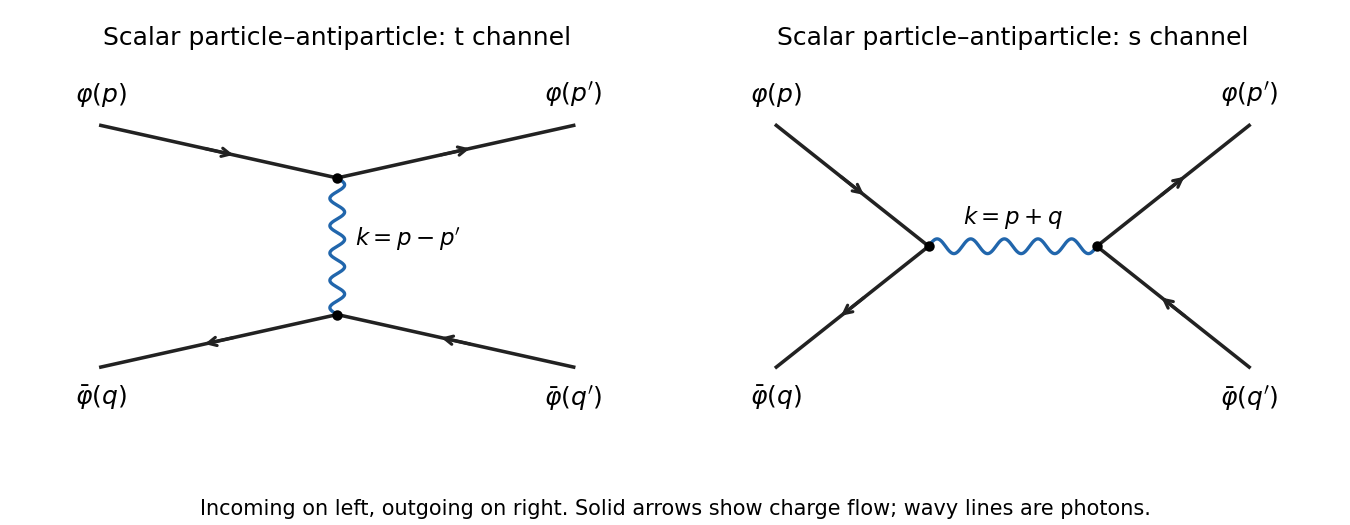
Leading scalar particle–antiparticle scattering diagrams with exchanged and annihilation-channel photons
. Details. 
For the exchange graph, let . Apart from overall charge signs, the two scalar currents are and . The external mass shell conditions giveFor the annihilation graph, , with currents and , again up to vertex signs. Their contractions are and . Thus each graph couples the photon to conserved currents, the relevant scalar quantum electrodynamics Ward identity.
Write and . conserved current means and . For , contraction with the Coulomb-gauge photon propagator gives, displaying the rational identity before the pole boundary limit,We used . Restoring the common Feynman i-epsilon prescription yields the Coulomb-gauge propagator between conserved currents resultHence each on-shell tree amplitude can use the Lorentz-invariant propagator. This is equality after contraction, not equality of the gauge-dependent tensors. At , the separate Coulomb-gauge terms are ill-defined; combine them first and take the conserved-current limit. The combined expression has only the physical photon pole.
Antiparticles are positive-energy quanta of relativistic quantum fields, not physical particles with negative energies. The negative-frequency part of a quantum field creates these quanta; the distinction between its classical frequency and a state's excitation energy is central to their interpretation.
For a real scalar field, Hermiticity identifies the two frequency branches:There is one species of excitation. Its particle is its own antiparticle; a single Hermitian scalar cannot carry the nonzero continuous phase charge of a complex field. This does not prevent self-conjugate particles from having other quantum numbers.
A complex scalar field is not Hermitian. Its two independent sets of oscillators giveThe canonical commutation relations make and create different positive-energy species. With charge convention fixed by , normal ordering givesThus and have the same mass and spin but opposite charge. Although has negative classical frequency, , so it creates a positive-energy excitation. Two real scalar fields can be combined into one complex field; the particle–antiparticle basis diagonalizes the conserved phase charge. Neutrality alone does not require a particle to be self-conjugate.
Locality explains why both branches occur. For the complex scalar field,At spacelike separation, Lorentz invariance of the mass shell measure permits a frame with equal times; reversing makes the two terms cancel. This is microcausality. If the antiparticle creation term were omitted, the commutator would be just a Wightman function, generally nonzero at spacelike separation. For example, for a massless scalar at equal times and separation , it is . The cancellation is the role of antiparticle modes and spacelike commutativity. In a real scalar field its self-conjugate creation modes supply the same cancellation.
A nonrelativistic particle field obeys a first-order time equation and need not contain an antiparticle-creation branch. For example,allows an expansion using only in ; its adjoint creates those particles. The basic theory conserves particle number and does not impose a Lorentz-invariant light cone locality condition. It often arises from a relativistic quantum field by factoring out the rest-energy oscillation and restricting to a low-energy particle sector, where creation of particle–antiparticle pairs costs roughly . An antiparticle species can certainly also be treated nonrelativistically with its own field; antiparticles are simply not forced by this nonrelativistic quantum field equation.
Historically, the Dirac equation has one-particle energy branches . Treating both as ordinary electron energies would leave no lowest-energy one-particle vacuum: an electron could fall through arbitrarily negative levels. The Dirac sea interpretation fills every negative-energy electron level. The Pauli exclusion principle then blocks further occupation. A missing negative-energy electron is a hole: removing energy increases energy by , and removing charge leaves charge . This predicts the positron's mass, spin and opposite electric charge.
The quantum field theory account quantizes a Dirac field instead:The independent particle and antiparticle operators obey canonical anticommutation relations. Before normal ordering, the negative-frequency contribution to the Dirac Hamiltonian has the form . Anticommutation rewrites it as plus a vacuum constant. Removing the constant leaves positive particle and antiparticle energies. The charge has opposite signs on the two occupation numbers, and interactions permit pair creation and annihilation while conserving the relevant charges.
There is therefore no need for a literal infinitely populated material sea. The hole picture is a useful fermionic reinterpretation, but it cannot explain bosonic antiparticles through filled-level exclusion, since bosons can multiply occupy a state. Canonical quantization of a complex scalar field supplies them just as consistently. More generally charge conjugation relates field representations with opposite internal charges; real scalar fields and Majorana fermions are self-conjugate exceptions. The relativistic Fock space description handles these cases, statistics and changing particle number within one framework.
Articles by others on the same topic
There are currently no matching articles.