Past exam of the mathematics course of the University of Cambridge / 2009 / iii / Paper 73 / 4

Set $S={\partial }_z\overline{u}>0$ and $N^2=-(g/{\rho }_0){\partial }_z\overline{\rho }>0$, using the constant reference mass density ${\rho }_0$ of the Boussinesq approximation. The mean-shear production is $\mathcal{P}=-\overline{u^{\prime }{w}^{\prime }}S>0$. The stable buoyancy destruction is $B=(g/{\rho }_0)\overline{{\rho }^{\prime }{w}^{\prime }}>0$. ThereforeThe Flux Richardson number compares stable buoyancy destruction with shear production; the gradient Richardson number compares restoring stratification with mean shear rate. They are generally different. The stationary energy budget gives $ϵ=\mathcal{P}(1-{\mathrm{Ri}}_f)$, so positive dissipation in this balance requires ${\mathrm{Ri}}_f<1$.

The fluctuation speed $q$ and the integral scale of turbulence $L_u$ give a turnover time $L_u/q$. Dividing the velocity-variance scale $q^2$ by that time gives a turbulent kinetic energy dissipation rate proportional to $q^3/L_u$. Likewise mass density variance $\overline{{\rho }^{\prime 2}}$ removed over scalar mixing time $L_{\rho }/q$ gives the density-variance dissipation rate proportional to $\overline{{\rho }^{\prime 2}}q/L_{\rho }$. Absorbing dimensionless proportionality coefficients into the specified length scales givesThese are integral-scale closure estimates, not exact consequences of dimensional analysis alone. In particular $q^2=2k$ for the turbulent-energy convention in Question 3. The normalization of $\chi$ is the one fixed by the printed scalar balance; if the budget is written for the full variance rather than one half of it, both production and dissipation terms acquire a factor two.

Write $F=\overline{{\rho }^{\prime }{w}^{\prime }}$. The density-variance balance gives $F{\overline{\rho }}_z=-\overline{{\rho }^{\prime 2}}q/L_{\rho }$. From the definition of $C_{\rho }^2$, $\overline{{\rho }^{\prime 2}}=F^2/(C_{\rho }^2{q}^2)$. For a nontrivial stratified turbulent state, substitute and divide by $F$:This is positive for the stipulated stable negative mass density gradient. The mean-shear production is $\mathcal{P}=C_u{q}^{2}S$. Substitute the scalar flux and $ϵ=q^3/L_u$ into $\mathcal{P}=B+ϵ$ to obtainEquivalently $C_{u}S{q}^2=C_{\rho }^2{L}_{\rho }{N}^{2}q+q^3/L_u$. This is the fixed-correlation equilibrium model for stratified turbulence. The unstratified limit has $F=0$ and is obtained by continuity without performing the division by $F$ at zero. The mass density symbols in the actual PDF are $\rho$; the converted TeX's pressure-like $p$ symbols in this equation are transcription errors.

For $q>0$, divide the two sink terms by $\mathcal{P}=C_{u}S{q}^2$. PutThe requested ratio isHere $b>0$ and $a\ge 0$. With stable stratification $a>0$, $R$ diverges at both $q\downarrow 0$ and $q\to \infty$, and has a single minimum at $q_m=\sqrt{a/b}$, with $R_{\min }=2\sqrt{ab}$. Increasing the stable density-gradient magnitude increases $a$, lifting the minimum and moving it rightward. When the mass density gradient vanishes, $a=0$ and the curve reduces to the straight line $R=bq$, with zero only as a limiting value at $q=0$ where the original ratio is undefined.

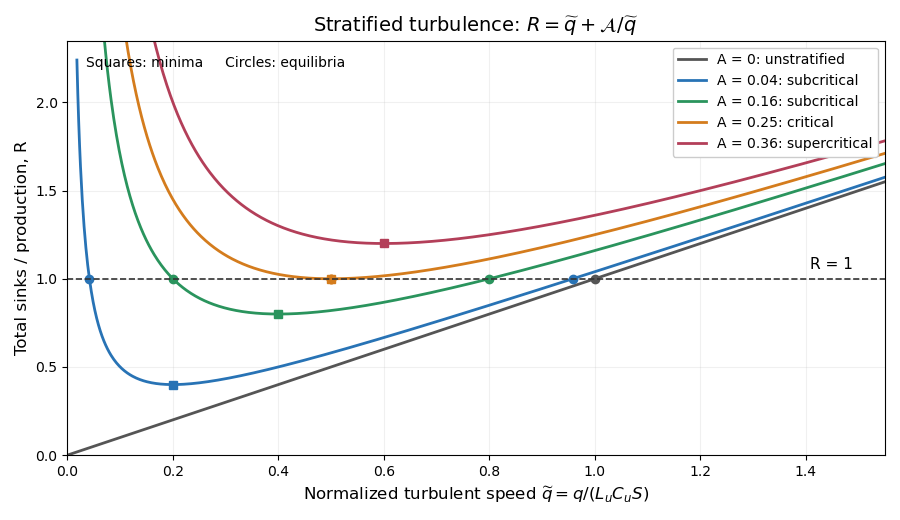
The plot uses $\tilde{q}=bq=q/(L_u{C}_{u}S)$ and $\mathcal{A}=ab=[L_{\rho }{C}_{\rho }^2/(L_u{C}_u^2)]\mathrm{Ri}$, so $R=\tilde{q}+\mathcal{A}/\tilde{q}$. The horizontal line $R=1$ selects equilibria: two positive intersections for $0<\mathcal{A}<1/4$, one double intersection at $\mathcal{A}=1/4$, and none above it. The zero-gradient line has one positive equilibrium; its formal zero root before division by $q$ is the non-turbulent state.

Differentiating $R=a/q+bq$ gives $R^{\prime }=-a/q^2+b$, so for positive stratification its minimum has $q_m^2=a/b$. At that pointThus the two sinks are equal. The buoyancy fraction of total turbulent sinks is always $B/(B+ϵ)=1/2$ there. But the Flux Richardson number defined in part (i) is insteadIt equals $1/2$ only when the minimum is also an equilibrium, $R_{\min }=1$, namely at the critical gradient. This is the qualification needed for the printed assertion; an arbitrary minimum on a curve plotted away from equilibrium need not have ${\mathrm{Ri}}_f=1/2$.

For example choose closure parameters $C_u=C_{\rho }=1/4$, units with $L_u=L_{\rho }=S=1$, and $N^2=1/16$. Then $a=1/64$, $b=4$, $q_m=1/16$ and $R_{\min }=1/2$. The actual flux Richardson number at this minimum is $1/4$, while the buoyancy fraction of the total sinks is $1/2$. This is a concrete counterexample to the unqualified wording. With zero mass density gradient there is no positive interior minimum at all, and ${\mathrm{Ri}}_f=0$.

Divide the equilibrium equation by $q>0$ to get $b{q}^2-q+a=0$. Hence both positive branches, when $0<4ab<1$, areAt equilibrium, ${\mathrm{Ri}}_f=a/q=1-bq$. Therefore the larger-speed branch $q_{+}$ gives the printed flux Richardson numberwhile the smaller-speed branch gives the same formula with a plus sign before the square root. Solving the quadratic alone does not discard that second branch.

The larger-speed branch is selected by local kinetic-energy stability. If the same closures are used in the local energy evolution, $\frac{1}{2}d(q^2)/dt=\mathcal{P}-B-ϵ$. For $q>0$, divide by $q$ to obtainIts linearization at $q_{\pm }$ has derivative $C_{u}S-2q_{\pm }/L_u=\mp C_{u}S\sqrt{1-4ab}$. The upper branch is therefore stable and the lower unstable in this local closure model.

The discriminant gives the critical gradient Richardson numberAt criticality the branches meet and ${\mathrm{Ri}}_f=1/2$. At zero stratification the stable positive solution is $q=C_{u}S{L}_u$ with ${\mathrm{Ri}}_f=0$; the lower algebraic root is $q=0$. This closure-dependent critical value is not automatically the inviscid $1/4$ criterion of the Miles–Howard theorem.

For $\mathrm{Ri}>{\mathrm{Ri}}_c$, the fixed-correlation equilibrium model for stratified turbulence has $R_{\min }>1$. Thus buoyancy destruction plus dissipation exceeds shear production for every $q>0$, and the local kinetic-energy budget predicts decay rather than any positive statistically steady turbulent equilibrium. The stable and unstable turbulent branches have disappeared together at the critical point.

The implied outcome within this closure is suppression or decay of sustained turbulence. It is not a proof that every physical stratified shear flow above this value must be permanently laminar: energy transport, external forcing, intermittent mixing or variable correlations and length-scale ratios can violate the model assumptions. As turbulence decays, the original fully turbulent high-Reynolds-number approximation itself ceases to apply. The critical Richardson number is consequently a prediction of the stated local closure, not a universal nonlinear stability bound.