Past exam of the mathematics course of the University of Cambridge / 2009 / iii / Paper 73 (Fluid Dynamics of Energy)

Choose $x$ upslope and $z$ normally downwards from the impermeable roof, so the buoyant layer occupies $0<z<h(x,t)$. Use the hydrostatic approximation and neglect the ambient return-flow pressure correction of relative order $h/H$. Pressure continuity at the interface gives the pressure inside the buoyant layer asThe along-slope Darcy velocity is thereforeDefine $u=kg\Delta \rho \sin \theta /\mu$. Integrating over depth gives the volume flux per unit width $F=uh-u\cot \theta h{h}_x$. Local fluid-volume conservation, including porosity, is $\varphi h_t+F_x=0$. Hence the inclined porous gravity current satisfiesThe first term is upslope advection driven by the mass density difference; the second is nonlinear hydrostatic spreading. The Darcy velocity $u$ and the corresponding pore velocity $u/\varphi$ must be distinguished.

When the hydrostatic spreading term is small, the depth equation reduces to $h_t+c{h}_x=0$, where $c=u/\varphi$. Its characteristic curves have $x=c(t-t_0)$, and the depth is constant along each characteristic. At the inlet the imposed flux gives $uh(0,t_0)=Q{e}^{-t_0/\tau }$. Therefore $h_0=h(0,0)=Q/u$ in this advective approximation andThis is the advection limit of an inclined porous current, behind its leading nose and after the relevant characteristic has left the inlet. For injection starting into an empty aquifer, the advective support is $0<x<ut/\varphi$.

The qualification “sufficiently large time” must refer to an advection-dominated outer region, not an exact solution of the full nonlinear equation. Substituting this exponential into the full equation leaves a nonzero spreading term. The next part quantifies when it can be neglected and explains the nonuniform leading-edge limit.

For the proposed exponential profile, put $\ell =u\tau /\varphi$. Then $h_x=h/\ell$ and $(h{h}_x{)}_x=2h^2/{\ell }^2$. Thus the exact ratio of the discarded spreading term to the retained advective term isThis is a quantitative validity condition for the advection limit of an inclined porous current. For a specified small tolerance $\eta >0$, at a fixed $x$ it is enough that the inlet characteristic has arrived andIf the logarithm is negative, arrival itself already gives this tolerance. A large-distance estimate comparing the overall current length $ct$ with a height-induced pressure length $h\cot \theta$ is $t\gg \varphi h\cot \theta /u$, but the local gradient criterion above is the sharper test for this particular injection history.

At the advective nose, $x=ut/\varphi$, the exponential factor is one. Therefore large time alone is insufficient for uniform validity: the outer profile also needs $2\varphi h_0\cot \theta /(u\tau )\ll 1$, and its abrupt nose needs an inner spreading layer. This limitation follows by direct substitution, not from a missing constant in the solution.

Indeed, with $\xi =x-ut/\varphi$, the full equation becomes $h_t=D(h{h}_{\xi }{)}_{\xi }$, $D=u\cot \theta /\varphi$. Once a finite-volume injection pulse is effectively over, nonlinear diffusion continues to broaden it. Dimensional balances give width ${\ell }_d\sim (DMt{)}^{1/3}$ and height $M/{\ell }_d$, where $M=\int hd\xi$ is the conserved area. A fixed exponential translating profile cannot be the uniform infinite-time limit of that equation. The printed formula is consequently an outer advection approximation with the displayed smallness condition.

Let $X(t)$ be the advancing nose into previously unoccupied pores. In the advective limit the interior flux is $uh$, while the exterior current thickness and flux are zero. Applying the Rankine-Hugoniot condition to the storage $\varphi h$ givesThis is the leading-edge kinematic boundary condition. The outer depth immediately behind this nose is $h(X(t{)}^{-},t)=h_0$, whereas ahead it is zero. A first-order advection model allows this jump; imposing zero depth on its interior trace would contradict its characteristic solution.

For the full inclined porous gravity current, the nose is instead resolved by a continuous spreading layer with $h(X,t)=0$. Taking the flux divided by depth at that interface gives $\dot{X}=(u/\varphi )(1-\cot \theta h_x{|}_{X^{-}})$, when this one-sided derivative exists. Its leading outer value is $u/\varphi$ only when the nose correction is negligible on the scale of the approximation. The zero-depth condition belongs to that resolved layer, not to the discontinuous outer profile itself.

At a fixed location behind the advancing nose, the depth decreases after passage. A fall $-dh>0$ leaves the immobile fluid volume $s\varphi (-dh)$ per unit length, so total local fluid storage changes by $\varphi dh+s\varphi (-dh)=\varphi (1-s)dh$. The thinning-region equation is thereforeThe inlet flux remains $uh(0,t)=Q{e}^{-t/\tau }$. Applying the method of characteristics with thinning-wave speed $u/[\varphi (1-s)]$ gives the residual-trapping attenuation of a porous current:The nose advances into new pore space, which has no residual fluid yet, so its storage factor is still $\varphi$ and its speed is still $u/\varphi$. Consequently $X(t)=ut/\varphi$ and the interior nose trace becomes $h_0{e}^{-st/\tau }$. Using the faster thinning-wave speed for the leading nose would incorrectly erase the attenuation caused by capillary residual trapping. The broken printed reference “(??)” points to the preceding outer profile.

The mobile fluid volume per unit well length includes the porosity:Integrating the residual-trapping attenuation of a porous current gives, for $0\le s<1$,This is mobile volume in the current; retained fluid outside its mobile thickness is not counted. Since $h_t=-h/\tau$ in the thinning region, the rate of accumulation of immobile retained volume is ${\dot{V}}_r=sV/\tau$. Direct differentiation verifies $\dot{V}+{\dot{V}}_r=Q{e}^{-t/\tau }$, so the mobile-volume expression obeys the overall injection balance.

Without capillary residual trapping, $s=0$ gives $V=Q\tau (1-e^{-t/\tau })$. The limiting expression as $s\to 1$ is $V=Qt{e}^{-t/\tau }$, though the local thinning equation degenerates at exactly $s=1$. Both limits provide useful consistency checks.

For $0<s<1$, differentiation givesIts unique zero solves $e^{-(1-s)t/\tau }=s$. Therefore the mobile-volume peak of an exponentially forced porous current occurs atThe derivative is initially positive and is negative after this time. More explicitly, at the stationary point $V^{\prime \prime }=-Qs{e}^{-st/\tau }/\tau <0$. Thus it is the global positive maximum, withThe claim of a finite maximum requires nonzero capillary residual trapping. At $s=0$ the mobile volume rises monotonically towards $Q\tau$ and the peak time tends to infinity. As $s\to 1$, the limiting peak time is $\tau$ and the limiting maximum is $Q\tau /e$.

Let $X(t)$ denote the polymer–oil material interface, measured from the injection well, and let $U(t)$ be the Darcy velocity. Incompressibility and uniform cross-sectional area make $U$ independent of $x$ in this planar model. Integrating Darcy's law through the injected layer and the oil layer givesThe material interface moves at the pore velocity, so $X^{\prime }=U/\varphi$. Put $a=\mu -{\mu }_h$ and $A={\mu }_{h}L$. Then $(A+aX)X^{\prime }=k\Delta P/\varphi$, which integrates from $X(0)=0$ toThus the fixed-pressure planar Darcy displacement hasFor $a\ne 0$, $X=[\sqrt{A^2+2ak\Delta Pt/\varphi }-A]/a$; its continuous $a=0$ limit is $X=k\Delta Pt/(\varphi {\mu }_{h}L)$. Positive layer dynamic viscosities ensure the resistance stays positive until breakthrough, which occurs at $t_b=\varphi L^2(\mu +{\mu }_h)/(2k\Delta P)$. The formulas stop there, since the two-layer geometry then changes.

Let $Y(t)$ be the porous thermal front and $X(t)$ the polymer front. With the literal stated convention for Darcy velocity,Therefore $Y=\beta X$ with $\beta =\Gamma \varphi$. This is thermal-front retardation in Darcy flow. The region $0<x<Y$ is cold injected fluid of dynamic viscosity $\mu$; $Y<x<X$ is heated injected fluid of dynamic viscosity $b\mu$; $X<x<L$ is oil of dynamic viscosity ${\mu }_h$. The pressure drop is consequentlywhere ${\mu }_{\mathrm{eff}}=\mu [\beta +b(1-\beta )]$. Apply the preceding fixed-pressure planar Darcy displacement calculation with $\mu$ replaced by this effective dynamic viscosity. The polymer-front speed isIts position solves ${\mu }_{h}LX+({\mu }_{\mathrm{eff}}-{\mu }_h)X^2/2=k\Delta Pt/\varphi$, and $Y=\Gamma \varphi X$. These expressions hold while both interfaces remain in the field, the porous thermal front is sharp and stable, and $0\le \Gamma \varphi \le 1$. For $b=1$ the original constant-viscosity answer is recovered.

Sometimes a thermal retardation factor is defined relative to the pore velocity instead. Under that alternative definition one substitutes $\beta =\Gamma$ throughout. The factor of $\varphi$ in the boxed answer follows specifically from the PDF's phrase “fraction of the Darcy speed.”

At the porous thermal front, the cold polymer solution behind has dynamic viscosity $\mu$, while the hot solution ahead has dynamic viscosity $b\mu >\mu$. Thus a more mobile region pushes a less mobile one. A forward protrusion locally reduces the length of high-resistance hot fluid and concentrates Darcy flux into itself; it advances faster, amplifying the protrusion. This is the mechanism of the Saffman–Taylor instability.

The leading polymer–oil interface can nevertheless be stable when the hot polymer dynamic viscosity is at least the oil dynamic viscosity. Stability of that leading interface does not guarantee stability of the trailing porous thermal front. Slow thermal conduction makes the latter sharp and offers weak short-wave smoothing; in practice it is the adverse dynamic viscosity contrast across this front that can invalidate the assumed planar stable-flow calculation.

Take constant Darcy velocity $U$ and work locally near a planar porous thermal front moving at $V_T=\Gamma U$. Let $\xi =x-V_{T}t$ and perturb its position by $\eta ={\eta }_0{e}^{\sigma t+iay}$, with wavelength $\lambda =2\pi /|a|$. Neglect thermal conduction and regard the adjoining layers as semi-infinite on this disturbance scale. In each region, Darcy's law and incompressibility imply that the pressure perturbation is harmonic, so the bounded normal modes areHere the minus side is cold with dynamic viscosity $\mu$, and the plus side is hot with dynamic viscosity $b\mu$. The base pressure gradients are $p_{-,x}^0=-\mu U/k$ and $p_{+,x}^0=-b\mu U/k$. Linearizing pressure continuity at the displaced front yieldsContinuity of the perturbed normal Darcy velocity givesso $A_{+}=-b{A}_{-}$. Therefore $\delta U=U|a|(b-1){\eta }_0/(b+1)$. The thermal-front kinematic law is $\sigma {\eta }_0=\Gamma \delta U$, proving the thermal-front viscous-fingering dispersion relationIt is positive for $b>1$, zero for $b=1$, and negative for $b<1$. Without thermal conduction the model has no finite fastest wavelength: the positive growth rate increases without bound as $\lambda \to 0$. A resolved thermal transition and diffusion regularize that short-wave limit.

For a material interface the kinematic coefficient would be $1/\varphi$ rather than $\Gamma$. Thus, if the interface of interest were instead the hot polymer–oil interface, the same calculation would give $\sigma =2\pi (U/\varphi )({\mu }_h-b\mu )/[\lambda ({\mu }_h+b\mu )]$, the usual planar viscous-fingering dispersion relation. This distinguishes the two interfaces and their speeds. The boxed thermal result uses the local planar approximation; distant wells or the other front modify the pressure eigenfunctions for wavelengths comparable to those separations.

Here $k$ is turbulent kinetic energy per unit mass, $k=\frac{1}{2}\overline{u^{\prime 2}+v^{\prime 2}+w^{\prime 2}}$, rather than the permeability of a porous medium used in the porous-flow questions. The K-epsilon turbulence model represents the high-Reynolds-number transport of this energy and its turbulent kinetic energy dissipation rate $ϵ$.

In the $k$ equation, $d[({\nu }_T/{\sigma }_k)k_y]/dy$ is the divergence of modeled turbulent diffusion, $\mathcal{P}$ is mean-shear production, and $-ϵ$ is molecular conversion of fluctuation energy into heat. Statistical stationarity and fully developed flow have removed storage and streamwise advection from this reduction.

In the $ϵ$ equation, $d[({\nu }_T/{\sigma }_{ϵ}){ϵ}_y]/dy$ transports dissipation intensity; $C_{ϵ1}\mathcal{P}ϵ/k$ models its generation associated with energy production; and $-C_{ϵ2}{ϵ}^2/k$ models its destruction. The time scale $k/ϵ$ supplies the source-rate dimension. The $ϵ$ equation is a closure, not another energy-conservation equation. Finally, ${\nu }_T=C_{\mu }{k}^2/ϵ$ has dynamic viscosity dimensions and parametrizes Reynolds stress transport; ${\sigma }_k,{\sigma }_{ϵ}$ set the relative diffusion strengths, and the remaining constants calibrate the closure.

Let the mean streamwise velocity be $U(y)$ and set $S=dU/dy>0$. The relevant covariance is $\overline{u^{\prime }{v}^{\prime }}<0$ on this half of the channel. The work of the Reynolds stress against the mean shear rate givesThe eddy viscosity relation is $-\overline{u^{\prime }{v}^{\prime }}={\nu }_{T}S$, soThese are the kinematic-stress conventions, with the covariance measured per unit mass; inserting a stress measured in force per area would require division by mass density.

The law of the wall in the logarithmic overlap region is $U/u_{\ast }={\kappa }^{-1}\log (y/y_0)+B$, with the wall-scale reference absorbed in $y_0$ and $B$. Differentiating gives the mean shear rateHere $\kappa$ is the Von Kármán constant. This form applies outside the viscous sublayer but well below the outer channel scale; it is not valid at the wall itself or at the channel centre.

Define the friction velocity by $u_{\ast }=(|{\tau }_w|/\rho {)}^{1/2}$, where ${\tau }_w$ is the total tangential wall stress. It is a stress-derived velocity scale, not the local mean velocity. In the overlap region, $y$ is small relative to the channel half-width, so the total stress is approximately its wall value. Molecular stress is small there, giving $-\overline{u^{\prime }{v}^{\prime }}\simeq u_{\ast }^2$.

Combining this Reynolds stress with the logarithmic shear gives $\mathcal{P}\simeq u_{\ast }^3/(\kappa y)$. For locally equilibrated wall turbulence, energy transfer to small scales occurs over the local eddy turnover time and is balanced by molecular dissipation; energy storage and the net energy-transport divergence are small in the leading overlap-layer balance. ThusThis is the local turbulent kinetic energy balance. It is a modeling approximation rather than a general identity for all wall positions. The constant-energy solution derived next is consistent with it: its modeled $k$ diffusion term is exactly zero, while the $ϵ$ diffusion term remains essential.

The constant Reynolds stress and the logarithmic shear imply the eddy viscosity ${\nu }_T=u_{\ast }\kappa y$. On the other hand the K-epsilon model gives ${\nu }_T=C_{\mu }{k}^2/ϵ$. Insert $ϵ=u_{\ast }^3/(\kappa y)$:Canceling the positive factors yields $C_{\mu }{k}^2=u_{\ast }^4$. Since energy is nonnegative, the log-layer solution of the k-epsilon model hasindependent of $y$ to this leading overlap-layer accuracy. In particular $k_y=0$, and the $k$ diffusion term vanishes, confirming the local production–dissipation balance in the energy equation.

Equating the two expressions for eddy viscosity gives directlyFrom the preceding part, $u_{\ast }^2=\sqrt{C_{\mu }}k$. Replace one factor of $k$ using that identity, and then replace $u_{\ast }$ itself by $C_{\mu }^{1/4}{k}^{1/2}$. This proves all three equivalent dissipation expressions:Each is the same turbulent kinetic energy dissipation rate, with dimensions of velocity cubed divided by length. Its equivalent friction-velocity form is $u_{\ast }^3/(\kappa y)$.

Use ${\nu }_T=u_{\ast }\kappa y$, $ϵ=u_{\ast }^3/(\kappa y)$, $k=u_{\ast }^2/\sqrt{C_{\mu }}$, and $\mathcal{P}=ϵ$ in the dissipation equation. Its diffusion term isThe net modeled source is $(C_{ϵ1}-C_{ϵ2}){ϵ}^2/k=-(C_{ϵ2}-C_{ϵ1})\sqrt{C_{\mu }}{u}_{\ast }^4/({\kappa }^2{y}^2)$. Dividing the equation by $u_{\ast }^4/y^2$ and solving givesThe physical Von Kármán constant is the positive root, requiring $C_{ϵ2}>C_{ϵ1}$ with positive $C_{\mu },{\sigma }_{ϵ}$. Neglecting dissipation diffusion would incorrectly require the two dissipation-equation constants to be equal. The parameter ${\sigma }_k$ does not enter because the constant $k$ profile has no energy-diffusion contribution.

Set $S={\partial }_z\overline{u}>0$ and $N^2=-(g/{\rho }_0){\partial }_z\overline{\rho }>0$, using the constant reference mass density ${\rho }_0$ of the Boussinesq approximation. The mean-shear production is $\mathcal{P}=-\overline{u^{\prime }{w}^{\prime }}S>0$. The stable buoyancy destruction is $B=(g/{\rho }_0)\overline{{\rho }^{\prime }{w}^{\prime }}>0$. ThereforeThe Flux Richardson number compares stable buoyancy destruction with shear production; the gradient Richardson number compares restoring stratification with mean shear rate. They are generally different. The stationary energy budget gives $ϵ=\mathcal{P}(1-{\mathrm{Ri}}_f)$, so positive dissipation in this balance requires ${\mathrm{Ri}}_f<1$.

The fluctuation speed $q$ and the integral scale of turbulence $L_u$ give a turnover time $L_u/q$. Dividing the velocity-variance scale $q^2$ by that time gives a turbulent kinetic energy dissipation rate proportional to $q^3/L_u$. Likewise mass density variance $\overline{{\rho }^{\prime 2}}$ removed over scalar mixing time $L_{\rho }/q$ gives the density-variance dissipation rate proportional to $\overline{{\rho }^{\prime 2}}q/L_{\rho }$. Absorbing dimensionless proportionality coefficients into the specified length scales givesThese are integral-scale closure estimates, not exact consequences of dimensional analysis alone. In particular $q^2=2k$ for the turbulent-energy convention in Question 3. The normalization of $\chi$ is the one fixed by the printed scalar balance; if the budget is written for the full variance rather than one half of it, both production and dissipation terms acquire a factor two.

Write $F=\overline{{\rho }^{\prime }{w}^{\prime }}$. The density-variance balance gives $F{\overline{\rho }}_z=-\overline{{\rho }^{\prime 2}}q/L_{\rho }$. From the definition of $C_{\rho }^2$, $\overline{{\rho }^{\prime 2}}=F^2/(C_{\rho }^2{q}^2)$. For a nontrivial stratified turbulent state, substitute and divide by $F$:This is positive for the stipulated stable negative mass density gradient. The mean-shear production is $\mathcal{P}=C_u{q}^{2}S$. Substitute the scalar flux and $ϵ=q^3/L_u$ into $\mathcal{P}=B+ϵ$ to obtainEquivalently $C_{u}S{q}^2=C_{\rho }^2{L}_{\rho }{N}^{2}q+q^3/L_u$. This is the fixed-correlation equilibrium model for stratified turbulence. The unstratified limit has $F=0$ and is obtained by continuity without performing the division by $F$ at zero. The mass density symbols in the actual PDF are $\rho$; the converted TeX's pressure-like $p$ symbols in this equation are transcription errors.

For $q>0$, divide the two sink terms by $\mathcal{P}=C_{u}S{q}^2$. PutThe requested ratio isHere $b>0$ and $a\ge 0$. With stable stratification $a>0$, $R$ diverges at both $q\downarrow 0$ and $q\to \infty$, and has a single minimum at $q_m=\sqrt{a/b}$, with $R_{\min }=2\sqrt{ab}$. Increasing the stable density-gradient magnitude increases $a$, lifting the minimum and moving it rightward. When the mass density gradient vanishes, $a=0$ and the curve reduces to the straight line $R=bq$, with zero only as a limiting value at $q=0$ where the original ratio is undefined.

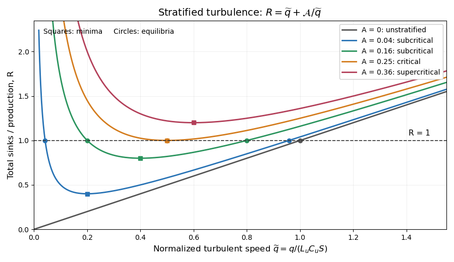
The plot uses $\tilde{q}=bq=q/(L_u{C}_{u}S)$ and $\mathcal{A}=ab=[L_{\rho }{C}_{\rho }^2/(L_u{C}_u^2)]\mathrm{Ri}$, so $R=\tilde{q}+\mathcal{A}/\tilde{q}$. The horizontal line $R=1$ selects equilibria: two positive intersections for $0<\mathcal{A}<1/4$, one double intersection at $\mathcal{A}=1/4$, and none above it. The zero-gradient line has one positive equilibrium; its formal zero root before division by $q$ is the non-turbulent state.

Differentiating $R=a/q+bq$ gives $R^{\prime }=-a/q^2+b$, so for positive stratification its minimum has $q_m^2=a/b$. At that pointThus the two sinks are equal. The buoyancy fraction of total turbulent sinks is always $B/(B+ϵ)=1/2$ there. But the Flux Richardson number defined in part (i) is insteadIt equals $1/2$ only when the minimum is also an equilibrium, $R_{\min }=1$, namely at the critical gradient. This is the qualification needed for the printed assertion; an arbitrary minimum on a curve plotted away from equilibrium need not have ${\mathrm{Ri}}_f=1/2$.

For example choose closure parameters $C_u=C_{\rho }=1/4$, units with $L_u=L_{\rho }=S=1$, and $N^2=1/16$. Then $a=1/64$, $b=4$, $q_m=1/16$ and $R_{\min }=1/2$. The actual flux Richardson number at this minimum is $1/4$, while the buoyancy fraction of the total sinks is $1/2$. This is a concrete counterexample to the unqualified wording. With zero mass density gradient there is no positive interior minimum at all, and ${\mathrm{Ri}}_f=0$.

Divide the equilibrium equation by $q>0$ to get $b{q}^2-q+a=0$. Hence both positive branches, when $0<4ab<1$, areAt equilibrium, ${\mathrm{Ri}}_f=a/q=1-bq$. Therefore the larger-speed branch $q_{+}$ gives the printed flux Richardson numberwhile the smaller-speed branch gives the same formula with a plus sign before the square root. Solving the quadratic alone does not discard that second branch.

The larger-speed branch is selected by local kinetic-energy stability. If the same closures are used in the local energy evolution, $\frac{1}{2}d(q^2)/dt=\mathcal{P}-B-ϵ$. For $q>0$, divide by $q$ to obtainIts linearization at $q_{\pm }$ has derivative $C_{u}S-2q_{\pm }/L_u=\mp C_{u}S\sqrt{1-4ab}$. The upper branch is therefore stable and the lower unstable in this local closure model.

The discriminant gives the critical gradient Richardson numberAt criticality the branches meet and ${\mathrm{Ri}}_f=1/2$. At zero stratification the stable positive solution is $q=C_{u}S{L}_u$ with ${\mathrm{Ri}}_f=0$; the lower algebraic root is $q=0$. This closure-dependent critical value is not automatically the inviscid $1/4$ criterion of the Miles–Howard theorem.

For $\mathrm{Ri}>{\mathrm{Ri}}_c$, the fixed-correlation equilibrium model for stratified turbulence has $R_{\min }>1$. Thus buoyancy destruction plus dissipation exceeds shear production for every $q>0$, and the local kinetic-energy budget predicts decay rather than any positive statistically steady turbulent equilibrium. The stable and unstable turbulent branches have disappeared together at the critical point.

The implied outcome within this closure is suppression or decay of sustained turbulence. It is not a proof that every physical stratified shear flow above this value must be permanently laminar: energy transport, external forcing, intermittent mixing or variable correlations and length-scale ratios can violate the model assumptions. As turbulence decays, the original fully turbulent high-Reynolds-number approximation itself ceases to apply. The critical Richardson number is consequently a prediction of the stated local closure, not a universal nonlinear stability bound.