Let be the one-dimensional turbulent energy spectrum, normalized so that . Large energy-containing eddies receive energy from the forcing. In the inertial range, nonlinear transfer passes this energy towards smaller scales at a mean rate per unit mass. Dimensional analysis of Kolmogorov 1941 theory givesThe dissipation range begins near the inverse of the Kolmogorov length scale, where kinematic viscosity removes the transferred kinetic energy. The large-scale spectrum depends on the forcing; the rising low- branch in this sketch is illustrative, rather than a universal power law.
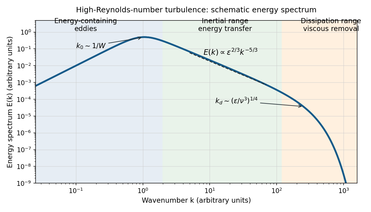
Schematic turbulence energy spectrum showing energy-containing eddies, the inertial range and viscous dissipation
. Details. 
The tube has neither homogeneous nor isotropic large-scale turbulence: gravity selects a vertical direction, its walls constrain the motion, and its density gradient varies with height. The width bounds the transverse size of the energy-containing eddies. At sufficiently high Reynolds number, much smaller eddies may become approximately locally isotropic and exhibit an inertial range, even though the full tube flow does not satisfy the homogeneous-isotropic assumptions.
To obtain the Reynolds stress, write and , with . Averaging the incompressible Navier-Stokes equations uses and gives the Reynolds-averaged momentum equationHere the final term is the mean buoyancy force, with the hydrostatic reference removed. Thus averaging the quadratic momentum flux introduces the covariance ; multiplied by , it has the dimensions of a stress. Its divergence transfers momentum between the mean flow and the fluctuations.
An eddy viscosity model represents this Reynolds stress byThe isotropic term can be absorbed into the mean pressure, while the deviatoric term gives a diffusion of mean momentum with turbulent viscosity , where and are representative turbulent speed and mixing length. Unlike kinematic viscosity, this coefficient depends on the flow. The closure assumes a local relation between stress and mean strain; anisotropic, buoyancy-driven large eddies may require a more detailed Reynolds stress model.
Write for the unstable, horizontally averaged density gradient. A turbulent displacement over a mixing length of order encounters a density contrast . Balancing its buoyancy acceleration with the inertial acceleration givesA turbulent diffusivity for density is therefore , absorbing dimensionless factors into . The upward density flux is : turbulent exchange carries denser water downwards and lighter water upwards. Defining as the positive downward flux yields the buoyancy-driven turbulent density diffusion lawThis is a flux per unit horizontal area, with units of mass per area per time. The total density transport across a horizontal section is .
The assumptions are established high-Reynolds number turbulence, width-limited eddies, an instantaneous local balance between buoyancy and inertia, approximately constant , negligible molecular diffusion, and zero mean vertical volume flux. The last condition follows from incompressibility and impermeable sidewalls in a closed tube. Density variations and the eddy statistics must also vary slowly enough for a local mixing-length closure to be meaningful.
Horizontal averaging of mass conservation, with upward , gives . Differentiating once more supplies the requested evolution of the density gradient:Under the Boussinesq approximation, replace in the inertial prefactor by the constant reference density ; retain the changing density gradient inside the flux.
In the Boussinesq approximation, put . The buoyancy-driven turbulent density diffusion equation gives, wherever ,The coefficient outside the bracket is positive, so the local density gradient increases precisely whenAt a point where , use the original degenerate diffusion equation rather than dividing by .
For the proposed self-similar solution, and . Substitution into givesAn odd power profile has right-hand spatial power . Matching it to requires . Thus choose with , an odd, increasing profile. Since , its flux is proportional to on both sides of the midplane. The resulting quintic density-profile similarity in an unstable tube satisfiesIntegration gives . ConsequentlyAlthough mixing transports density downwards, the local density gradient can grow because spatial variations of the flux redistribute density. In this example the downward flux increases towards each end, driving the formal amplification of the odd profile.
This self-similar solution deliberately ignores the end conditions: its nonzero end flux cannot satisfy impermeable ends. Moreover, the Boussinesq approximation requires , which fails before the formal divergence. A closed tube has only finite available potential energy, so it cannot sustain indefinitely growing turbulent kinetic energy or the assumed instantaneous flux law. End effects, changing eddy statistics and decay of the unstable stratification must eventually replace this local model. The conflicting endpoint labels in the source do not enter the calculation because end conditions have been expressly excluded.
Articles by others on the same topic
There are currently no matching articles.