Assume small-amplitude, nonrotating, inviscid Boussinesq approximation motion about a fluid at rest, with stable background stratification. In either uniform layer let be the buoyancy perturbation and . The linear equations areFor a plane internal gravity wave proportional to , continuity gives , and horizontal momentum gives . Substituting these into vertical momentum and buoyancy evolution givesChoose , . Its group velocity isThus downward energy propagation has . If is the acute angle between the ray and the vertical in its direction of propagation, then , soThe phase velocity is parallel to , while : phase and group velocities are perpendicular, and their vertical components have opposite signs. Propagating incident waves require ; both layers support propagating waves only when . At or above , the lower layer cannot carry a propagating downward internal wave.
For the amplitude convention used below, multiplies the unit particle-displacement vector along the ray, with positive horizontal component. That vector is for a downward wave and for an upward wave. Stating this polarization convention is important when assigning a sign to a reflection coefficient.
Time and horizontal translational invariance at the interface conserve and . For every component, horizontal momentum givesThe background density has the same value on both sides, so pressure continuity implies continuity of horizontal velocity. Normal velocity is also continuous: no fluid accumulates at the interface.
Use the particle-displacement amplitudes and polarization directions defined in part (a). For downward incident and transmitted waves and an upward reflected wave, continuity of and givesSolving the two equations proves the internal-wave transmission across a buoyancy-frequency jump formulaThe reflected wave has the same frequency and wavelength as the incident wave and opposite vertical wavenumber. The transmitted wave hasIts group velocity is downward at angle ; the formula in part (a), with , gives its speed.
If instead one uses signed vertical-displacement amplitudes, the reflected coefficient has the opposite sign: . This follows because the reflected polarization's vertical component changes sign, and is not a difference in the physical reflected field. As an energy check, the reflected fraction is and the transmitted fraction is ; they sum to one.
When , take , , so decays as . The transmitted field is evanescent, carries no mean vertical energy flux, and the reflected wave has unit amplitude magnitude. A real lower-layer ray angle and wavelength are then inapplicable.
The rigid bottom reflects the lower-layer wave. Its repeated returns to the interface create an internal-wave cavity response containing both upward and downward components in , while the upper layer contains the imposed incident wave and one net reflected wave.
Let the lower downward and upward particle-displacement coefficients be and , multiplying and respectively. Their vertical displacement has opposite polarization signs:Zero normal velocity at gives , where . Interface continuity consequently becomesFor the specified angles, and . ThusThe dependence on bottom depth is thereforeIn particular,Here and , so the positive depths giving this maximum areThe lower vertical-displacement standing-wave envelope is , while its horizontal-displacement envelope has the complementary cosine form. These distinguish the total standing disturbance from the amplitude of either traveling component. The traveling amplitude has minimum at .
Since , . Hence the net upward-propagating wave in the upper layer has amplitude magnitude for every , with the phase given above. At an enhancement maximum, and . No energy escapes through the bottom, so complete eventual reflection is consistent with energy conservation.
At a fixed time, the complete spatial derivative isThe first term describes geometric variation along the channel at a fixed surface elevation. The second describes the extra wetted area produced by a varying water level; is the surface width.
Assume a fixed channel, negligible lateral inflow, uniform cross-sectional velocity, incompressible water and the hydrostatic long-wave approximation. Integrating volume conservation over a short channel segment givesInviscid horizontal momentum, with measured from the fixed datum, is . The coefficient matrix acting on has eigenvaluesThese are the variable-section channel characteristics. Put . Adding the corresponding linear combinations of the two equations givesThe opposite signs in the two combinations cancel both derivative terms in the source calculation.
If , then and . Taking along a characteristic gives the requested formA sufficient geometry assumption is , for which is independent of at fixed height.
For a completely general , the printed form omits an explicit wave-speed geometry term. The correct conversion is insteadFor example, a lake at rest with constant but position-dependent has . The printed left side is then nonzero while its right side is zero. The -based compatibility equation remains valid, including when makes the speed-based expression singular.
Linearize about water at rest with uniform surface elevation . Write , , and . To first order the shallow water equations becomeDifferentiate continuity in time and eliminate :For a time-harmonic standing disturbance, use . ThenDividing by provesThis identifies the coefficient as the local long-wave wavenumber. It is constant under the fixed-shape geometry used in part (a), when is independent of ; that assumption is needed for the constant-coefficient mode calculation in part (c).
Assume is constant, as for constant resting long-wave speed. With , put . The amplitude equation becomesIf , write : the solution is an oscillatory sine-cosine combination multiplied by . If , it is . If , it is a combination of real exponentials, , where . These classify the local spatial behavior.
For a nonzero-frequency mode, zero velocity at both dams and impose . In the oscillatory case, the first condition givesIts derivative at is . Hence the standing modes in an exponentially tapered channel haveThe hyperbolic and repeated-root cases provide no additional nonzero-frequency mode satisfying both end conditions. There is a separate zero-frequency uniform-level mode , corresponding to a change of the basin's conserved water volume.
A failed dam launches a rarefaction wave back into the reservoir and an advancing current into the initially dry downstream channel. Take the failed dam as , initial depth and zero velocity for , and a dry bed for . Locally assume a flat, prismatic triangular section, . The early flow is governed byIts Riemann invariants are , since . In the left-running simple wave, , where , and the expanding fan has . Solving givesThus the triangular-channel dry-bed dam break profile isThe reservoir-side edge moves at , and the dry front moves atVelocity is zero in the undisturbed reservoir and has the fan value above where water is present. This approximation applies before the rarefaction reaches the surviving dam and before channel variation, friction or finite-volume reflections substantially modify the flow. If water is already present downstream, a bore replaces the dry-bed front and requires a different matching problem.
Take positive upward from the release and define the pressure scale height . Neglecting the small ambient density variation in the hydrostatic pressure calculation,Conservation of gas mass and Boyle's law giveHere to leading order in the dilute bubble concentration. If the thermal's total volume is , its bubble fraction and bubble contribution to reduced gravity areThus the volume-integrated kinematic buoyancy contribution is , and the corresponding upward force is approximately times this quantity. Bubble expansion increases this total contribution even while entrainment dilutes the local concentration.
Neglect bubble rise relative to the water when the bubbles' terminal slip speed is much smaller than the thermal rise speed, their response time is short compared with , and they remain well dispersed and retained. Small bubbles are more likely to satisfy these conditions; large bubbles can escape through the thermal. The approximations also require , , negligible gas dissolution and no important surface-tension correction. Pressure must remain positive and the hydrostatic expression is used only below the ocean surface.
The Boussinesq approximation retains small density differences only in the gravitational buoyancy force and uses a constant reference density in inertia and volume conservation. The entrainment coefficient specifies the inward velocity of ambient fluid relative to the thermal boundary, . Turbulent interface motions engulf ambient water and mix it into the coherent rising volume.
For a spherical buoyant thermal, . To leading order in the dilute gas fraction, expansion of the gas does not dominate the total-volume balance, so fluid entrainment givesBut and . Therefore, wherever the thermal is rising,This growth law for a dilute bubbly thermal is independent of stratification under the constant- model. Stratification changes the speed and eventual stopping height; it does not enter this volume-per-distance relation. In real flows the entrainment coefficient itself can vary with stratification and flow structure.
For a high-Reynolds number thermal, buoyancy force scales as and inertial resistance scales as . Their balance gives . It is therefore natural to write a diameter-based Froude number closureThe order-one coefficient accounts for the thermal's shape, entrainment and flow structure. The main resistance is inertial pressure or form drag and the momentum needed to entrain and accelerate surrounding water, rather than molecular skin friction. Added mass matters when the thermal accelerates, so the Froude closure is a quasi-steady approximation.
In a homogeneous ocean all of the leading buoyancy comes from the bubbles. Parts (a) and (b) giveSubstituting into the speed law yieldsFor , this becomesThe square root is essential both physically and dimensionally. This approximation still requires dilute bubbles and retained gas; it is not a valid prediction of infinite speed where the pressure approximation approaches zero.
For constant buoyancy frequency in the Boussinesq approximation, the ambient density isConservation of liquid mass during fluid entrainment gives , with . Integrating by parts,Since and ,Hence the water density within the thermal isThe entrained water is denser than its new surroundings because it retains a mixture of fluid drawn from lower levels.
The bulk density is . Dropping products of the small density contrast with , its net reduced gravity isThe first term is the expanding-bubble contribution and the second is the restoring effect of stratification. In the quasi-steady Froude model, ascent stops when . The neutral height of a bubbly thermal in a stratified fluid therefore satisfiesThis is a fifth-degree polynomial, with leading coefficient at finite release pressure. The relevant height is the first positive zero reached while the thermal is still below the surface, dilute and within the Boussinesq range. Depending on parameters there may be no such zero before the surface, or more than one mathematical zero; a later root beyond a first stopping point is not another continuous ascent solution. The model's stopping height is a neutral-buoyancy estimate, not a claim that inertial overshoot is absent.
For a very deep release, over the rise, so bubble expansion is negligible. The neutral-height equation reduces toThusIf the stopping thermal is also much larger than its initial size, the leading form isThe first expression does not require this extra entrainment-dominated limit.
Near the neutral height the quasi-steady speed tends to zero. Momentum can produce some overshoot and subsequent adjustment or oscillation. The water spreads horizontally as a buoyant intrusion near its equilibrium density level. Bubble slip then becomes important relative to the slowing liquid, so bubbles can separate and continue rising toward the surface, reducing the residual liquid's buoyancy. Loss of bubbles and further mixing alter the final intrusion level; the retained-bubble model no longer applies indefinitely after stopping.
Let be the one-dimensional turbulent energy spectrum, normalized so that . Large energy-containing eddies receive energy from the forcing. In the inertial range, nonlinear transfer passes this energy towards smaller scales at a mean rate per unit mass. Dimensional analysis of Kolmogorov 1941 theory givesThe dissipation range begins near the inverse of the Kolmogorov length scale, where kinematic viscosity removes the transferred kinetic energy. The large-scale spectrum depends on the forcing; the rising low- branch in this sketch is illustrative, rather than a universal power law.
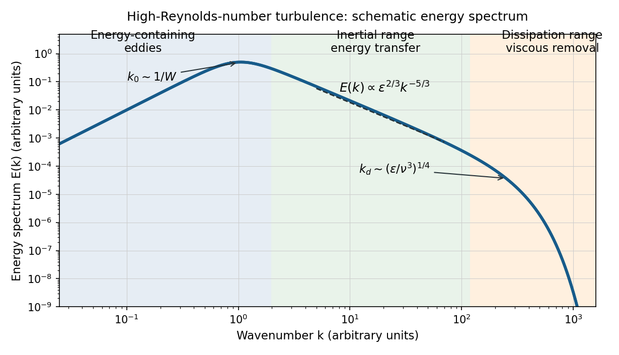
Schematic turbulence energy spectrum showing energy-containing eddies, the inertial range and viscous dissipation
. Details. 
The tube has neither homogeneous nor isotropic large-scale turbulence: gravity selects a vertical direction, its walls constrain the motion, and its density gradient varies with height. The width bounds the transverse size of the energy-containing eddies. At sufficiently high Reynolds number, much smaller eddies may become approximately locally isotropic and exhibit an inertial range, even though the full tube flow does not satisfy the homogeneous-isotropic assumptions.
To obtain the Reynolds stress, write and , with . Averaging the incompressible Navier-Stokes equations uses and gives the Reynolds-averaged momentum equationHere the final term is the mean buoyancy force, with the hydrostatic reference removed. Thus averaging the quadratic momentum flux introduces the covariance ; multiplied by , it has the dimensions of a stress. Its divergence transfers momentum between the mean flow and the fluctuations.
An eddy viscosity model represents this Reynolds stress byThe isotropic term can be absorbed into the mean pressure, while the deviatoric term gives a diffusion of mean momentum with turbulent viscosity , where and are representative turbulent speed and mixing length. Unlike kinematic viscosity, this coefficient depends on the flow. The closure assumes a local relation between stress and mean strain; anisotropic, buoyancy-driven large eddies may require a more detailed Reynolds stress model.
Write for the unstable, horizontally averaged density gradient. A turbulent displacement over a mixing length of order encounters a density contrast . Balancing its buoyancy acceleration with the inertial acceleration givesA turbulent diffusivity for density is therefore , absorbing dimensionless factors into . The upward density flux is : turbulent exchange carries denser water downwards and lighter water upwards. Defining as the positive downward flux yields the buoyancy-driven turbulent density diffusion lawThis is a flux per unit horizontal area, with units of mass per area per time. The total density transport across a horizontal section is .
The assumptions are established high-Reynolds number turbulence, width-limited eddies, an instantaneous local balance between buoyancy and inertia, approximately constant , negligible molecular diffusion, and zero mean vertical volume flux. The last condition follows from incompressibility and impermeable sidewalls in a closed tube. Density variations and the eddy statistics must also vary slowly enough for a local mixing-length closure to be meaningful.
Horizontal averaging of mass conservation, with upward , gives . Differentiating once more supplies the requested evolution of the density gradient:Under the Boussinesq approximation, replace in the inertial prefactor by the constant reference density ; retain the changing density gradient inside the flux.
In the Boussinesq approximation, put . The buoyancy-driven turbulent density diffusion equation gives, wherever ,The coefficient outside the bracket is positive, so the local density gradient increases precisely whenAt a point where , use the original degenerate diffusion equation rather than dividing by .
For the proposed self-similar solution, and . Substitution into givesAn odd power profile has right-hand spatial power . Matching it to requires . Thus choose with , an odd, increasing profile. Since , its flux is proportional to on both sides of the midplane. The resulting quintic density-profile similarity in an unstable tube satisfiesIntegration gives . ConsequentlyAlthough mixing transports density downwards, the local density gradient can grow because spatial variations of the flux redistribute density. In this example the downward flux increases towards each end, driving the formal amplification of the odd profile.
This self-similar solution deliberately ignores the end conditions: its nonzero end flux cannot satisfy impermeable ends. Moreover, the Boussinesq approximation requires , which fails before the formal divergence. A closed tube has only finite available potential energy, so it cannot sustain indefinitely growing turbulent kinetic energy or the assumed instantaneous flux law. End effects, changing eddy statistics and decay of the unstable stratification must eventually replace this local model. The conflicting endpoint labels in the source do not enter the calculation because end conditions have been expressly excluded.
Let , and . The inviscid shallow water equations areTaking the vertical curl of the momentum equation, with constant , gives . Combining this with the depth equation provesThus shallow-water potential vorticity is materially conserved: changes in absolute vorticity are exactly compensated by stretching or compression of the layer depth.
The relation to a Bernoulli function presupposes steady flow. In that case define . The vector identity givesSteady volume conservation allows a transport stream function with . Hence , soIn particular, : the Bernoulli function is constant along each streamline. Where the flow permits a single-valued dependence on the stream function, the displayed derivative describes how that constant changes between neighbouring streamlines. For an unsteady flow, shallow-water potential vorticity remains conserved but the stated steady Bernoulli function relation does not generally hold.
Take from the first wall to the second, with . Negligible transverse velocity and cross-channel geostrophic balance give , since the bed elevation is independent of . Therefore the volume flux isFor positive downstream volume flux, the layer is deeper at the first wall: . This calculation does not require zero shallow-water potential vorticity.
Here must denote the wall depth above the local bed. If the surface heights are instead measured from a fixed vertical datum, write them as and use , giving . The compact formula thus uses a bed-relative meaning of the wall heights.
Material conservation of shallow-water potential vorticity carries from the reservoir into the channel. At leading order in a long, slowly varying channel, and are negligible, so . Zero absolute vorticity therefore implies . Integration from , followed by cross-channel geostrophic balance, gives the zero-potential-vorticity rotating channel flow:In particular, and . The velocity increases towards the shallower wall. Differentiating the depth-based specific energy confirmsThis cross-channel constancy is also the consequence of .
For a reservoir of finite depth, exact requires relative vorticity , an anticyclonic rotation cancelling the planetary vorticity. A reservoir at rest in the rotating frame has and , so it does not have exactly zero shallow-water potential vorticity. A very deep, nearly quiescent reservoir can nevertheless supply the approximation because is small. The idealization must describe vanishing absolute vorticity or this deep-reservoir limit, rather than ordinary finite-depth rest in the rotating frame.
Put and , the mean of the two wall velocities. The zero-potential-vorticity rotating channel flow has . Substitution into the volume flux formula givesThe resulting quadratic equation has two roots, . The positive-depth condition selects the minus sign. ThusThe discarded sign would make . On the retained branch , which also shows the admissibility condition .
The depth-based specific energy at the first wall isBecause , this same specific energy holds everywhere across the channel at fixed . Its sum with the bed elevation is the Bernoulli function divided by . Zero shallow-water potential vorticity makes that Bernoulli function constant throughout the connected steady channel flow, soConsequently the depth-based specific energy decreases as the bed rises and increases as it falls. It is constant along a level-bed channel, even if the width varies; that width variation instead changes the wall depths and velocities compatible with the conserved volume flux and Bernoulli function.
A hydraulic control of a zero-PV rotating channel is a critical section separating the upstream branch, where long-wave disturbances can propagate upstream, from the downstream branch, where they cannot. In the steady specific-energy description it is a stationary point of with respect to depth at fixed volume flux and local width. The control therefore fixes the discharge for a given upstream Bernoulli function and channel geometry; an arbitrary downstream condition cannot generally be imposed independently on the upstream reservoir.
Evaluate all quantities at and keep fixed while differentiating. With , the preceding branch givesAt the hydraulic control of a zero-PV rotating channel, this derivative vanishes. Using reduces it to , where . Equivalently,Combining this with cancels the quadratic term and leavesAt control and . Both walls must remain wet. Since , the second depth is positive precisely when , givingEquality is the limiting case , with the second wall just dry. For a wider channel, a dry lateral region requires a different solution and the two-wet-wall hydraulic control of a zero-PV rotating channel formula cannot be continued. The channel must also remain sufficiently long and slowly varying for the transverse geostrophic balance approximation to hold. As a check, gives , the familiar rectangular-channel critical discharge.
Articles by others on the same topic
There are currently no matching articles.