Assume and use geometric units. The stationary Killing vector field gives the conserved Killing energy . For radial motion, normalization of the four-velocity gives . Combining these identities yieldsAt rest at infinity, and , so . Choose the inward branch . Its proper time from the Schwarzschild event horizon to the curvature singularity isIn ordinary units this is . The endpoint is not a regular centre of the spacetime. This is the Schwarzschild horizon-to-singularity proper time for fall from infinity, rather than a universal time for all infall energies.
For this geodesic congruence, set . Its four-velocity and metric dual areThe right side is an exact one-form because depends only on . Thus , with free-fall proper time in Schwarzschild spacetime determined byIndeed , so this scalar advances by the actual proper time on every member of the infalling geodesic congruence, with a synchronized choice of additive offsets.
Substitution of in the Schwarzschild metric givesUsing , the Painlevé–Gullstrand coordinates therefore haveAll coefficients are finite at ; the determinant of the block is . Hence the horizon is a coordinate singularity of Schwarzschild time, not a degeneracy of the metric. The new spatial slices have , the flat Euclidean metric, and makes their normals the freely falling four-velocities. By contrast, the curvature scalar diverges at ; this genuine singularity is not removed.
For ingoing Eddington-Finkelstein coordinates, use with , for example . ThenBoth constructions cross the future horizon. Their time functions have different meanings: is an ingoing null hypersurface, whereas is a flat spacelike hypersurface orthogonal to the infallers. Thus the former is adapted to ingoing null geodesics, and the latter to a timelike free-fall clock congruence.
For the Kruskal diagram, choose Kruskal–Szekeres coordinates with , in the right exterior and extend them across its horizon. They obeyThe four regions of Kruskal spacetime are I, the right exterior ; II, the future black hole ; III, the other exterior ; and IV, the past white hole . The null axes are horizons, their intersection is the bifurcation two-sphere, and the spacelike boundaries are the future and past curvature singularities. A point in this radial diagram represents a symmetry two-sphere.
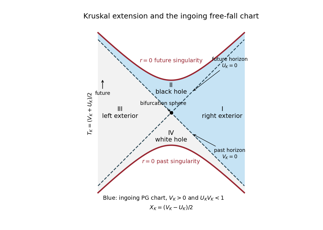
Kruskal extension with both exteriors, black hole and white hole; the ingoing Painlevé-Gullstrand domain is shaded blue
. Details. 
The domain of the ingoing Painleve-Gullstrand chart is region I together with region II and their common future horizon. More precisely, it is , , or with finite . To verify the boundary rather than infer it from the locally regular metric, put and writeThis follows by subtracting from the preceding radial primitive, and is finite at . Thus throughout the chart. Conversely every point with and gives a finite . The past horizon , the bifurcation sphere, region III and region IV are absent. Reversing the sign of the radial term produces the outgoing chart through the white hole instead.
Articles by others on the same topic
There are currently no matching articles.