Use an acoustic velocity potential with and . It obeys the wave equation . The rigid walls require zero normal velocity, hence Neumann boundary conditions on the transverse variables. Separation givesDefine . The dispersion relation, phase velocity and group velocity for positive areFor a dispersive mode, , decreases from infinity to , and increases from zero to . The mode has and : it propagates without dispersion.
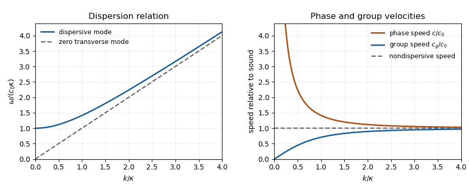
Acoustic waveguide dispersion and velocities; a nonzero transverse wavenumber is compared with the nondispersive mode
. Details. 
Let be the cross-sectional area. The appropriate time and cross-sectional average at fixed isWrite for the product of cosines and . Its transverse eigenvalue and wall conditions give by integration by parts. The kinetic energy density and compressive acoustic energy density are and . Time averaging each squared real oscillation contributes a factor , soThis holds for every dispersive mode, and also for the zero mode.
For localized smooth initial data, a dispersive mode contains integrals of the form along . When , a stationary point exists at . It is nondegenerate because . The stationary phase method therefore gives an oscillatory amplitude for each excited dispersive mode, and for their sum under sufficient mode summability.
At , no dispersive mode has a finite stationary wavenumber; with smooth localized data these contributions decay, while the nondispersive right-moving pulse retains its original amplitude. Thus a general disturbance with nonzero zero-mode component has an undiminished pulse on the sound-speed ray. If that component is absent, this surviving contribution is absent too. For , finite propagation speed puts a compactly supported initial disturbance outside this ray for all sufficiently large , so the field is eventually zero. Rapidly localized, rather than strictly compact, data give a correspondingly negligible tail instead.
Articles by others on the same topic
There are currently no matching articles.