Use the horizontal streamfunction convention , and set , . Geostrophic balance gives , henceThe constant is fixed by the total volume or the reference surface height. To obtain shallow-water quasi-geostrophic potential vorticity, require a small Rossby number, nearly geostrophic horizontal motion and . Expanding the exact shallow-water potential vorticity givesAt leading nontrivial order , so after removing the constant background and multiplying by ,The mean potential vorticity and its gradient areWith and , expand the Jacobian. Since both mean fields depend only on , their Jacobian vanishes. The two mixed terms are and , givingThe PDF has this correct mean-advection term; the TeX aid incorrectly inserts a division by .
Drop the quadratic perturbation Jacobian. Freeze and locally for a short-wave plane wave, with and . Then , , and the local Rossby-wave dispersion relation in a zonal jet isThe intrinsic phase moves against an eastward mean flow because .
The printed wavelength bound is not a consequence of these equations. The local short-wave assumption is , equivalently wavelength ; a particular cutoff is an optional scale-separation criterion, not a universal derived threshold. If one requires the ground-frame phase to follow the mean current, the dispersion relation only gives , or wavelength less than . For example has wavelength and a phase moving with the mean. More decisively, the stationary condition requested next fixes wavelength , contradicting a bound if both are imposed on the same waves.
For nonzero zonal and mean velocity, a ground-stationary wave satisfiesIt has the background length scale, so its existence should not be justified solely by the short-wave approximation. It is nevertheless an exact stationary linear solution of the Rossby-wave equation for a sheared zonal current: writing gives , which reduces to . Thus with works globally. Indeed the total field then has a constant, so its full Jacobian vanishes as well.
Differentiating the local dispersion relation givesOn the stationary circle this becomesFor a purely zonal wavevector, , this is the printed expression . With the printed expression needs a directional qualification; the general vector is the one above. Here stationarity means in the ground frame, not vanishing intrinsic frequency in the moving fluid.
A stationary obstacle can therefore anchor the phase pattern while wave energy travels away from it. The zonal group component has the mean-flow sign, so an eastward jet carries the stationary wave response downstream; tilted wavevectors also carry energy meridionally. This is the usual stationary Rossby wave wake distinction between fixed phase crests and propagating wave energy.
Let denote the signed vertical component of the Coriolis parameter; it is negative in the southern hemisphere. In the steady, linear, inviscid interior, depth integration of horizontal momentum giveswhere and . Horizontal curl eliminates the pressure. Its left side is . Incompressibility and impermeable flat top and bottom imply , givingThis is Sverdrup balance. It assumes steady small-amplitude motion, a Boussinesq approximation, negligible nonlinear advection, negligible Rayleigh and bottom/lateral drag in the interior, a flat fixed-depth domain and no normal top/bottom flux. The applied surface wind stress remains a forcing, even though interior friction is neglected. With cooling absent, the steady buoyancy equation additionally requires , if that equation is imposed; the curl balance itself does not depend on the cooling coefficient. In the closed, -independent channel below, depth-integrated , so a nonzero wind-stress curl cannot be balanced by an inviscid interior alone.
Steady forced channel. Now take . Put , and write for the positive wind-stress amplitude. The prescribed profiles giveThe buoyancy jumps across the sharp forcing interface in this simplified model; pressure and the circulation below are continuous. Let , , and . Hydrostatic balance gives . The horizontal momentum equations and their solution areThe no-normal-flow conditions imply : this integral is independent of by incompressibility and is zero at the meridional walls. It determines the otherwise free depth-uniform pressure gradient,DefineA meridional overturning streamfunction satisfying , isIt vanishes on all four boundaries. Together with the expressions for , this solves all the steady equations. The formula permits variable ; freezing it at a negative gives the simple schematic . No unspecified latitude dependence is silently needed for the sketch.
Since , upper-layer meridional transport is northward and the deep return is southward. At constant , the circulation rises on the southern side and sinks on the northern side. The meridional velocity changes sign at , slightly above the forcing interface, not exactly at . The required schematic follows from this derived field:
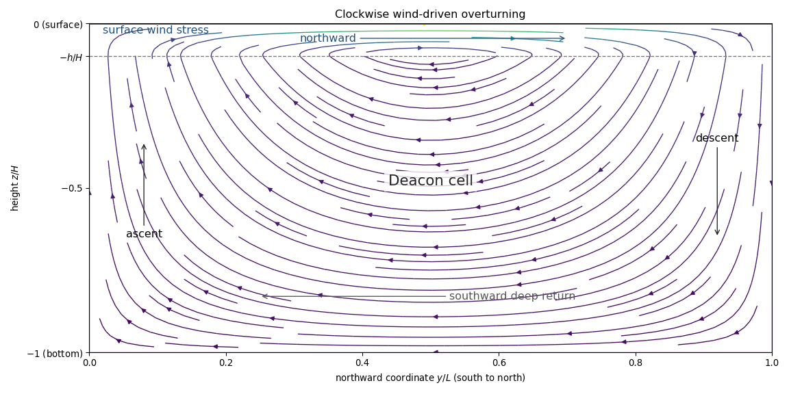
Clockwise Deacon circulation: northward surface transport, southward deep return, ascent in the south and descent in the north
. Details. 
Forcing comparison. The buoyancy and wind contributions have the same vertical shape and, with these signs, the same circulation sense. Their ratio isThe printed scaling must be understood in magnitude, since and both forcing amplitudes are positive. Surface confinement supplies the small factor , making direct buoyancy forcing negligible in this circulation model.
The missing physical mechanism in the stratified Southern Ocean is eddy-induced overturning. The wind-driven mean Deacon cell tilts isopycnals and builds available potential energy; baroclinic instability produces mesoscale eddies whose buoyancy transport largely opposes the mean overturning. The residual circulation depends on the small net balance and the diabatic buoyancy transformation. Wind energy also enters mean kinetic energy; eddies redistribute momentum through form stress and transfer energy toward dissipative scales and bottom friction. The displayed linear model already balances its wind input by imposed drag, but omits this mean-advection/eddy buoyancy budget, so the necessity of an opposing eddy circulation is a physical extension, not another mathematical constraint on the four given equations.
Define the positive total shear stress by , so the physical wall traction on the fluid opposes the positive flow. The steady mean momentum equation givesFor a driving pressure gradient , the stress decreases upward. It is approximately constant whileAn outer boundary-layer height can impose a stricter limit. In the turbulent region outside the viscous or roughness sublayer, the only local neutral scales are and , so . Conventionally write , where is the von Kármán constant. Equivalently, a mixing length and stress closure give the same result. Integration yields the law of the wallThe roughness length is an extrapolation scale, not a statement that the logarithm is valid at the actual solid surface. For a smooth boundary, the viscous inner scales are , . The viscous sublayer has ; farther out , corresponding to . For a fully rough boundary, is proportional to a geometric roughness height and viscosity no longer determines the leading profile. The logarithmic region still needs roughness height .
In local equilibrium, production of turbulent kinetic energy by the shear is . Neglecting its transport relative to production and viscous dissipation,Dimensional similarity alone gives ; the displayed coefficient additionally uses the local energy balance and the logarithmic shear.
Let be the vertical turbulent buoyancy flux, positive for heating from below. Its dimensions are length squared per time cubed. The stress velocity and height therefore admit a new dimensionless group . Define the signed Obukhov lengthStable cooling has ; unstable heating has . Monin-Obukhov similarity theory expresses the mean shear asThe similarity hypothesis assumes approximately steady, horizontally homogeneous, constant-stress and constant-flux conditions, with the observation level outside the inner sublayer but below the outer-layer scales. Dimensional analysis fixes the arguments and prefactor, not the entire function . A measured or modeled turbulence closure supplies its form.
For a rough boundary, integrate the similarity shear from the roughness length. A usual moderate-stability closure iswith positive dimensionless coefficients. These are empirical closures, not quantities determined by similarity alone. An often-used choice is . The unstable quarter-power relation is tested over approximately in Dyer's flux-gradient study; the stable coefficient convention is recorded in the surface-flux formulation. Near neutrality one takes their smooth limits.
For moderate stable conditions, integration givesFor the unstable closure set and defineThen andFor weak unstable departure, , this reduces to the stable-form expression with replaced by and a negative . The full quarter-power expression is useful for moderately unstable conditions with of order one; it must not be extrapolated automatically to the distinct asymptotic free-convection regime. The stable linear expression similarly describes a continuously turbulent surface layer, rather than guaranteeing validity after strong stratification destroys the constant-flux state. Both profiles require and approximately uniform fluxes.
At fixed friction velocity, unstable heating gives and . The usual similarity closure has , so it reduces the mean velocity gradient relative to the neutral law of the wall. Rising warm and descending cool parcels mix momentum efficiently; less mean shear is needed to transport the same stress. Relative to a fixed near-wall reference, the speed difference aloft is reduced.
Stable cooling gives and . The restoring buoyancy suppresses vertical parcel excursions and reduces the effective momentum diffusivity, requiring a steeper shear for the same stress. The speed difference from the wall reference is correspondingly larger. These are comparisons at prescribed stress; fixing an outer wind instead would allow and the stress to change, so it would not be the same comparison.
Write and . The gradient Richardson number and Flux Richardson number areThe first compares the restoring buoyancy gradient with mean shear; the second is the fraction of shear production consumed by stable buoyancy work. With this convention, both are positive for stable mixing and negative for unstable stratification. In local steady equilibrium, , so a positive dissipation requires . The inviscid Miles–Howard theorem concerning is a linear stability criterion, not a universal equality for turbulent fluxes.
Use the gradient-diffusion closures and . The turbulent Prandtl number is , givingUnder the ideal Reynolds analogy , the two Richardson numbers coincide. It is an additional closure, not an automatic consequence of the definitions. If the buoyancy-gradient similarity function is defined by , then
For lower-boundary heating, forced convection means that mean shear supplies most of the turbulence even though buoyancy assists it, approximately . Free convection means buoyancy dominates, approximately within the constant-flux region. In this limit the local convective speed isIt is the velocity whose eddy transport supplies the imposed vertical turbulent buoyancy flux. The associated diffusivity is , with a dimensionless coefficient fixed by a closure. From ,Here : there is no real restoring buoyancy frequency. The displayed magnitude is a local overturning/growth rate, or one may write . The Reynolds analogy makes and hence ; the remaining mean shear is weak compared with the convective motion.
The turnover dissipation estimate givesalso consistent with the local energy equation when is negligible. Thus free-convection dissipation is height independent to leading scaling order, in contrast with neutral . The constants and detailed profiles are not determined by dimensional analysis. These are local free-convection surface-layer scalings, not a claim that an entire deep convecting layer has a uniform unstable mean buoyancy gradient.
For very stable continuously turbulent conditions, , local eddies lose leading dependence on their distance from the wall. In very stable surface-layer similarity, the dimensionless functions must therefore scale as and , with positive closure constants. Using givesThus the mean velocity is approximately linear in height and the real buoyancy frequency is approximately constant, . Under the Reynolds analogy, .
The local turbulent kinetic energy balance givesPositive dissipation requires . The turbulent energy-turnover length is of order , hence of order the Obukhov length, independent of observation height. A related buoyancy-limited length is . The Ozmidov length follows by equating an eddy turnover time with :These are turbulent turnover or buoyancy-transition scales. If “the scale at which dissipation occurs” means the actual viscous cutoff, molecular viscosity is also required: the Kolmogorov microscales giveWithout , the viscous length cannot be fixed by the supplied stress and flux alone. Separating it from the turbulent turnover length avoids confusing an energy-budget estimate with the molecular cutoff.
Finally,They become height-independent constants. The commonly used continuation gives and . This numerical value is a closure choice, not a deduction from units; setting would incorrectly leave zero dissipation. Extremely stable intermittent or collapsed turbulence need not satisfy this local-equilibrium model. The relation between the Obukhov and buoyancy-dissipation lengths in the local regime is also analyzed in Grachev and colleagues' similarity study.
Use a top-hat plume model per unit span. Define volume and kinematic momentum fluxes and , and set the pure-ice reduced gravity . The suspension buoyancy is . The supplied equations express vertical momentum conservation, conservation of relative enthalpy including latent heat, and conservation of excess salt, respectively. At the release height, prescribe compatible source volume/momentum, salt and enthalpy fluxes, or equivalent source width, velocity, composition and ice fraction; impose ambient entrained water at with no vertical momentum. A pure far-field similarity solution may instead be described using a virtual origin, but its singular near-origin values are not physical inlet conditions.
The missing balance is total mass, equivalently volume under the Boussinesq approximation. In a wall plume, only the exposed outer edge entrains, so the Batchelor entrainment hypothesis givesIf two free edges are intended, replace by everywhere; the numerical coefficient is a geometry convention. The glacier boundary itself has no normal flow. Local phase conversion does not add volume at retained Boussinesq order, and crystals are assumed to share the liquid velocity.
For a box of height , the upward momentum flux changes by . The ambient hydrostatic pressure has been subtracted; the remaining force is the suspension buoyancy . Entrained ambient water carries no vertical momentum, and drag is neglected, giving . Salt entering through the exposed edge is , so and thereforeThese control-volume derivations account for entrainment rather than treating as constant.
Thermodynamic elimination. Let the conserved excess enthalpy and salt fluxes be and :The ambient satisfies , while equilibrium in the ice-bearing plume givesSubstitute this temperature in the enthalpy invariant. Exact rearrangement givesThus, at dilute-crystal order,The ice-bearing wall-plume thermodynamic invariant fixes the leading advected ice volume and buoyancy flux from the source deficits. A rising ice-dominated branch requires . It is not determined from reduced gravity alone. The small- expansion also presumes finite source fluxes and no cancellation making the discarded terms comparable to .
The three remaining leading equations are , , and . Seek a similarity form in with , . Continuity gives , while momentum gives . Therefore . The coefficients obey , giving the self-similar ice-bearing wall plumeThe width grows linearly, the speed approaches a constant, and the crystals dilute inversely with height. This is a buoyancy-conserving wall line plume, with buoyancy supplied mainly by the ice fraction rather than a temperature anomaly. The dilute-crystal regime requires and lies away from the formal virtual-origin singularity. If all source flux deficits vanish, and this nontrivial rising branch does not exist. The exact thermodynamic invariants above, rather than their truncated version, are needed near a concentrated source.
Articles by others on the same topic
There are currently no matching articles.