Past exam of the mathematics course of the University of Cambridge / 2013 / iii / Paper 73 (Fluid Dynamics of Climate)

Put $P=p/{\rho }_0$ and use the downward buoyancy anomaly $b=g{\rho }^{\prime }/{\rho }_0$. This sign convention is required by the printed potential vorticity. The linear rotating Boussinesq approximation givesLet $D=u_x+v_y$ and $\zeta =v_x-u_y$. Horizontal divergence and curl give $D_t-f\zeta =-{\nabla }_H^{2}P$ and ${\zeta }_t=-fD=f{w}_z$. HenceThus the linear potential vorticity is a time-independent field fixed by the initial data. Differentiate the pressure identity twice. Using ${\zeta }_{tt}=-f(P_{zz}+b_z)$ and $b_{ztt}=-N^2(P_{zz}+b_z)$ gives ${\nabla }^2{P}_{tt}=(N^2-f^2)(P_{zz}+b_z)$. Combining terms,The linear pressure equation for rotating stratified flow has source $Q={\rho }_{0}f{N}^{2}q$. “Arbitrary” means that different initial potential-vorticity fields give different time-independent sources; it is not independent forcing that may vary in time. If buoyancy were instead defined upward as $-g{\rho }^{\prime }/{\rho }_0$, both appearances of its sign would change consistently. The pressure source represents the balanced component alongside propagating inertia-gravity waves.

For a nonzero-frequency Fourier mode proportional to $e^{i(kx+mz-\omega t)}$, the time-independent source has no oscillatory part. The pressure equation givesTake $k,m\ne 0$ and ${\omega }^2\ne f^2,N^2$ for the following pressure-amplitude formulas. With $P_0$ the amplitude of $p/{\rho }_0$, the momentum and buoyancy equations implyConsequentlybecause the numerator is $(k^2+m^2){\omega }^2-N^2{k}^2-f^2{m}^2$. Propagating linear inertia-gravity waves carry zero perturbation potential vorticity. In degenerate directions the division formulas must be replaced by the original linear equations, or interpreted by a regular limit; the zero-PV property of the nonzero-frequency wave component still follows from $q_t=0$. A steady balanced mode need not have zero potential vorticity.

For the positive-frequency branch and $K^2=k^2+m^2$, the wavefront-normal phase velocity and the group velocity areTheir scalar product vanishes since $k(k{m}^2)+m(-m{k}^2)=0$. Equivalently, the frequency is homogeneous of degree zero in the wave vector, and hence $\mathbf{k}\cdot {\nabla }_{\mathbf{k}}\omega =0$.

The vertical sign relation isIt is negative for the usual geophysical ordering $N>|f|$ and nonzero $k,m$. Thus vertical phase and energy propagation are opposite under that ordering; negative-frequency waves obey the same product relation. The PDF does not state this ordering, so its unconditional direction assertion needs qualification. For example, $N=1$, $f=2$, $k=m=1$ gives positive vertical components on the positive-frequency branch. If $N=|f|$ the group velocity vanishes, and in axial limiting directions one vertical component can be zero. Orthogonality is valid throughout, while strictly opposite nonzero vertical components need the stated nondegeneracy and $N>|f|$.

Let the vertical-velocity amplitude $W$ be real. A convenient inertia-gravity wave polarization, avoiding pressure denominators, isThe physical velocities and buoyancy are their real parts. The period-mean kinetic energy density and available potential energy density areThe latter follows from $A={\rho }_0{b}^2/(2N^2)$, or from $A={\rho }_0{N}^2{\xi }_z^2/2$ for vertical fluid displacement. The factor $1/4$ includes both the energy definition and the mean of a squared harmonic.

Using the dispersion relation,This energy partition of rotating internal waves shows that the printed request for ordinary kinetic/potential equipartition in the rotating case is false in general. An explicit counterexample is $f=1$, $N=2$, $k=m=1$, $W=1$, giving ${\omega }^2=5/2$, $⟨K⟩=3{\rho }_0/5$ and $⟨A⟩=2{\rho }_0/5$.

The valid modified oscillator balance isThe transverse rotational velocity is in quadrature with the in-plane motion, so it supplies an additional positive energy term on the displacement side of this oscillator balance. It remains physically kinetic energy, not gravitational potential energy. Ordinary kinetic/potential equipartition is recovered when $f=0$ or when the transverse amplitude vanishes. For a real harmonic wave the instantaneous total $K+A$ is constant at a fixed point: the coefficient of ${\cos }^2(kx+mz-\omega t)$ from in-plane motion equals the coefficient of ${\sin }^2$ from transverse motion and buoyancy. This consistency does not imply equality of their separate period means.

The shallow-water approximation requires depth much less than horizontal length, a homogeneous incompressible fluid, gentle surface/bottom slopes, and frequencies slow enough that vertical acceleration is negligible compared with gravity. Continuity gives $w\sim (H/L)U$, making vertical inertial acceleration smaller than the horizontal inertial scale by the aspect ratio. The vertical momentum equation therefore reduces to $p_z=-{\rho }_{0}g$. With constant atmospheric pressure,The horizontal pressure gradient is independent of depth. Linearizing about rest and retaining the leading depth-uniform horizontal motion givesTheir horizontal curl gives ${\zeta }_t=-f(u_x+v_y)$, soHere $\zeta =v_x-u_y$ is relative vorticity; the PDF sentence identifying $\eta$ as relative vorticity is a symbol error. This is the linear shallow-water potential vorticity anomaly; advection of that perturbation is second order.

In the adjusted state take alongshore independence, decay offshore, and an impermeable coast. Steady continuity gives $u=0$, and geostrophic balance gives $v=g{\eta }_x/f$. Assume $f>0$ so the printed $a=\sqrt{gH}/f$ is a positive barotropic deformation radius. For either hemisphere the decay length is $\sqrt{gH}/|f|$, with the corresponding change in current direction. Initial rest makes the conserved anomaly $-{\eta }_{\mathrm{initial}}/H$, and thereforeThe coastal adjustment of an elevated strip uses a decaying offshore solution and a particular solution in the elevated strip are matched with continuous $\eta$ and $v$, hence continuous ${\eta }_x$, at $x=-L$. Integrating this equation over $x<0$ and conserving the initial volume per alongshore length, ${\int }_{-\infty }^0\eta dx={\eta }_{0}L$, gives $a^2{\eta }_x(0)=0$. Solving those matching conditions yieldsExpanding the hyperbolic functions gives exactly the alternative summed form in the PDF. Both matching values at $-L$ are ${\eta }_0(1-e^{-2L/a})/2$, and the wall elevation is ${\eta }_0(1-e^{-L/a})$.

The adjusted flow isThus both velocity components vanish at the coast. In this inviscid problem tangential no-slip is not generally an independently imposed wall condition; here it follows from initial rest and alongshore uniformity. Indeed $v_t+fu=0$ at the impermeable wall keeps $v(0,t)=0$. The mass constraint recovers the same adjusted-state condition.

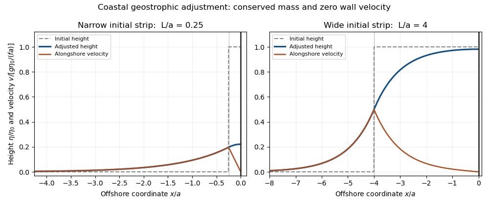
For $L\gg a$, the surface retains nearly its initial elevation through most of the strip. The offshore edge is smoothed over width of order $a$, with half-height at the original edge, while the coast remains at nearly ${\eta }_0$. The current is concentrated near the smoothed edge and vanishes at the coast.

For $L\ll a$, the elevation spreads over a much larger offshore scale $a$, with wall height approximately ${\eta }_{0}L/a$. Away from the thin original strip, $\eta \simeq {\eta }_0(L/a)e^{x/a}$. Within it the leading elevation is nearly that reduced constant, with a small curvature required to bring $v$ to zero at the wall. Wide strips retain a broad high plateau; narrow strips spread into a low deformation-scale coastal bulge. The total anomalous volume remains ${\eta }_{0}L$ in both limits.

Take a beta-plane approximation, $f=f_0+\beta y$ with $\beta >0$, and define the depth transport $\mathbf{T}=(U,V)={\int }_{-H}^0{\mathbf{u}}_{h}dz$. For steady flow with no net flux through surface and bed, depth-integrated continuity gives $U_x+V_y=0$. Vertical integration of momentum givesIn the interior, small depth-to-horizontal aspect ratio makes vertical stress divergence the leading viscous contribution; horizontal viscous terms are neglected there. Taking the vertical component of curl eliminates pressure. Sinceneglecting bottom stress gives the Sverdrup balance,Thus the wind-stress curl sets the interior meridional depth transport, not the local surface meridional velocity. A constant-$f$ plane would have no $\beta V$ term; the use of $\beta$ in this question requires latitude-dependent $f$. For a transport streamfunction with $(U,V)=(-{\bar{\psi }}_y,{\bar{\psi }}_x)$, the interior relation is $\beta {\bar{\psi }}_x=W/{\rho }_0$.

To close a depth-integrated bottom-drag model, approximate the bottom horizontal velocity by the depth mean, ${\mathbf{u}}_b\simeq \mathbf{T}/H$. This is the barotropic closure needed to express the stated stress solely in terms of the transport. DefineThe coefficient $\gamma$ in a physical stress law is not itself a drag rate; $r$ has units of inverse time. The ocean basin equation with bottom drag and lateral viscosity follows by taking curl of the integrated momentum equation and yields the combined Stommel boundary layer and Munk boundary layer equation,The bottom contribution is negative because the vertically integrated stress difference is surface stress minus bottom stress. Set the constant wall streamfunction to zero. No normal flow and no tangential slip impose $\bar{\psi }=0$ and ${\partial }_n\bar{\psi }=0$ on the walls.

The inviscid interior solution has ${\bar{\psi }}_I=S(y)x/\beta +C_0(y)$. In a thin east/west layer, $x$ derivatives dominate the smaller $y$ derivatives. Holding $y$ as a parameter givesEquivalently the boundary correction $\varphi =\bar{\psi }-{\bar{\psi }}_I$ obeys $\nu {\varphi }^{\prime \prime \prime \prime }-r{\varphi }^{\prime \prime }-\beta {\varphi }^{\prime }=0$. In a stretched inward coordinate $X=x/\delta$ at the west wall and $X=(1-x)/\delta$ at the east wall, this becomes respectivelyThe first-derivative sign reversal distinguishes east from west. Vanishing $W$ and its derivatives at the north/south boundaries makes leading forcing-dependent solutions compatible with those boundaries, avoiding extra leading meridional layers. These are leading boundary-layer equations, not an exact deletion of every meridional derivative in the full basin PDE.

The nonconstant exponential modes of the leading basin equation satisfyThus a leading uniformly valid form is $\bar{\psi }\simeq S(y)x/\beta +C_0(y)+{\sum }_{j=1}^3{C}_j(y)e^{{\lambda }_{j}x}$, with exponentials referenced to the wall where they decay. The coefficients enforce the four east/west no-slip conditions; their values are not needed to identify the scales.

If $r^3\ll {\beta }^2\nu$, horizontal viscosity dominates drag in the boundary layers. The Munk boundary layer scale is ${\delta }_M=(\nu /\beta {)}^{1/3}$, assumed much smaller than basin width. The roots are ${\delta }_M^{-1}$ and $(-1\pm i\sqrt{3})/(2{\delta }_M)$ to leading order, soThe east layer has exponential thickness ${\delta }_M$ and the west oscillatory layer has envelope thickness $2{\delta }_M$, both of order ${\delta }_M$. The west correction supplies the order-one return transport, while the east no-slip correction is typically smaller in amplitude. Setting $r=0$ still leaves enough viscous modes to impose no-slip.

If $r^3\gg {\beta }^2\nu$, linear drag dominates the broad vorticity layer. Definewith ${\delta }_S$ small compared with basin width. The roots are approximately $-{\delta }_S^{-1}$ and $\pm {\delta }_v^{-1}$; the fast roots have smaller correction $\beta /(2r)$. The drag-dominated basin solution with no-slip layers isThere is a broad western Stommel boundary layer of thickness ${\delta }_S$, a thinner western no-slip layer of thickness ${\delta }_v$, and an eastern no-slip layer of thickness ${\delta }_v$. The narrow layers can have small streamfunction amplitude while supplying an order-one change in wall velocity.

If viscosity is set identically to zero, only the particular solution, a constant and the western Stommel exponential remain. That second-order model cannot generally satisfy both streamfunction and derivative conditions at both walls. Small nonzero viscosity must be retained in the wall skins when no-slip is required. In the question's stress notation, the limits compare $[\gamma /({\rho }_{0}H){]}^3$ with ${\beta }^2\nu$. Neither limit applies at the crossover, where all cubic terms contribute. These composite forms are leading asymptotic solutions of the basin problem; meridional derivatives and interior diffusion supply higher-order corrections.

Use small Rossby number $U/(f_{0}l)\ll 1$, slow evolution on the advective time scale, small interface displacements relative to each layer depth, shallow hydrostatic layers, stable reduced gravity $g^{\prime }>0$, and inviscid unforced flow. On a beta plane, take $\beta l/f_0$ of the same small order as the Rossby number. The internal Burger number is retained at order unity so stratification and relative-vorticity effects can both enter the leading potential-vorticity anomaly.

The rigid-lid pressure in two-layer flow comes from neglecting the free-surface volume displacement in the rigid-lid approximation; it does not permit setting the common horizontal pressure gradient to zero. The small surface displacement multiplied by $g$ retains a finite lid-pressure multiplier. Write $h_1=H_1+\chi$, $h_2=H_2-\chi$, and let $\Pi$ denote this common pressure potential. Leading geostrophic balance giveswith ${\mathbf{u}}_i=(-{\psi }_{iy},{\psi }_{ix})$ at leading order. Literally setting $h_1+h_2$ to a spatial constant in the momentum gradients before taking the rigid-lid limit would suppress the upper-layer pressure field and fail to produce general two-layer QG dynamics.

Taking curl of each shallow-water momentum equation and using layer continuity gives material conservation of $(f+{\zeta }_i)/h_i$. Expanding it to first order and advecting the anomaly by the leading geostrophic velocity yieldsThe two-layer quasi-geostrophic potential vorticity equations areHere the common background $f_0/H_i$ has been removed and the anomaly multiplied by $H_i$. The advection term is retained at the same slow order as the time derivative even though the leading velocity/pressure balance was linear geostrophy. On an $f$ plane simply set $\beta =0$.

Let $d={\psi }_1-{\psi }_2$ and $C=f_0^2/g^{\prime }=H_1{F}_1=H_2{F}_2$. Multiply each two-layer quasi-geostrophic potential vorticity equation by $H_i{\psi }_i$ and sum. The time-derivative terms areThe interface terms combine to $-Cd{d}_t$, since the two layers share the same depth-weighted coupling $H_i{F}_i$. The planetary term $\beta y$ has no time derivative. For the nonlinear terms, ${\nabla }_h\cdot {\mathbf{u}}_i=0$ and ${\mathbf{u}}_i\cdot {\nabla }_h{\psi }_i=0$ implyConsequently the local two-layer quasi-geostrophic energy conservation law isThe flux expression is one convenient form obtained directly from the requested multiplication; divergence-free modifications would represent the same local balance. $E$ is physical energy per horizontal area divided by the common reference density. Multiplying both $E$ and ${\mathbf{F}}_E$ by that density restores the dimensional physical-energy convention.

Integrating the local two-layer quasi-geostrophic energy conservation law over a horizontal domain and using the specified vanishing boundary flux givesPeriodic boundaries, or suitable fixed streamfunction boundary data eliminating the displayed energy flux, provide examples. The gradient terms are the two layer kinetic energies; the last term is available potential energy, equal to $g^{\prime }{\chi }^2/2$ under the interface-displacement relation.

The baroclinic energy ratio and deformation scale for unequal layer depths uses a decomposition uses the depth-weighted barotropic streamfunction $\Psi =(H_1{\psi }_1+H_2{\psi }_2)/(H_1+H_2)$ and $d=2\tilde{\psi }$. Define $H_r=H_1{H}_2/(H_1+H_2)$. ThenFor variations on horizontal scale $l$, this givesFor comparable layer depths $H_r$ is of order either $H_i$, reproducing the requested scale $l^2{f}_0^2/(g^{\prime }{H}_i)$. If one layer is much thinner, its depth controls this ratio; a depth-independent arithmetic barotropic average would leave unwanted cross terms in the energy decomposition.

Baroclinic potential energy dominates at scales much larger than the two-layer internal deformation radius; baroclinic kinetic energy dominates at much smaller scales. They are comparable near $l\sim R_d$. The independent barotropic kinetic energy has no interface-displacement partner, so this scale comparison refers specifically to the baroclinic component.