Past exam of the mathematics course of the University of Cambridge / 2016 / iii / Paper 333 / 4

For steady depth and no sources of fluid mass, the continuity equation gives ${\nabla }_h\cdot (H\mathbf{u})=0$. In a simply connected region this defines an ocean transport streamfunction:A multiply connected basin additionally needs its circulation or boundary-constant data. Taking the vertical curl of $\mathbf{u}=(-{\psi }_y,{\psi }_x)/H$ gives the exact relative vorticity from a variable-depth transport streamfunction relationNo small-depth-variation expansion has been made. No normal flow at a basin wall means that $\psi$ is constant along that connected wall.

Let $Q_b=f/H$. At sufficiently small Rossby number, retain advection of this full background shallow-water potential vorticity while dropping the higher-order advection of $\zeta /H$. For uniform-depth Sverdrup balance, this also requires relative-vorticity advection to be small against planetary-vorticity advection; small Rossby number alone does not guarantee this when $\beta$ is very small. Multiplying the resulting steady potential vorticity equation by $H$ givesDefine the topographic potential-vorticity pseudovelocityIts sign is important: it is opposite to the coefficient vector on the left of the preceding equation. Substituting the ocean transport streamfunction expression for relative vorticity yieldsThe pseudovelocity follows contours of $f/H$ and is not the fluid velocity; its units are inverse length squared per time because $\psi$ is a transport streamfunction. If $r=F=0$, the ocean transport streamfunction is constant along each connected background potential vorticity contour. Locally, at regular points,with arbitrary differentiable $\Phi$. Different disconnected components of a level set may carry different functions until boundary conditions identify them. If $f/H$ is constant over an open region, the leading equation gives no restriction there; critical points similarly require regularity and global matching rather than division by a vanishing gradient.

For uniform depth on a beta plane, $\tilde{\mathbf{u}}=(-\beta /H,0)$. With weak bottom drag the equation reduces to Sverdrup balance,Restore a dimensional forcing amplitude $F_0$; the printed unit-amplitude forcing means $F_0=1$ in the chosen units. The general interior ocean transport streamfunction isTaking $\psi =0$ on a straight eastern boundary $x=x_e$ sets $C=0$; without a zonal boundary condition the function $C(y)$ remains arbitrary. ThenThe Sverdrup balance interior cannot satisfy both zonal-wall conditions; a western boundary current supplies the return circulation.

For basin scales $L_x,L_y$, use $V_S=F_0/\beta$, $U_S=V_S{L}_x/L_y$, and ${\Psi }_S=H{V}_S{L}_x$. The ratio of drag to Sverdrup balance terms is of orderThis criterion applies away from boundary layers and zeros of the leading forcing, with positive $H$, $\beta \ne 0$, and the beta plane and small-Rossby number assumptions. For an approximately square basin it is $r/(\beta L)\ll 1$. Neglect of nonlinear relative-vorticity advection further requires $U_S/(\beta L^2)\ll 1$ for comparable velocity and length scales. Thus weak drag relative to the balance, rather than just a small absolute $r$, is the appropriate condition.

Put $X=x-x_0$, $Y=y-y_0$ and take $\beta ,r,H>0$. The constant-depth ocean transport streamfunction equation isIt is a steady advection-diffusion equation for the transport response, with westward pseudovelocity. For an unbounded domain the point-forced Sverdrup–drag Green function can make its contours precise. Set $a=\beta /(2r)$ and $\psi =e^{-aX}\varphi$. Thenwhere $K_0$ is the Modified Bessel function of the second kind. This optional explicit expression is used only to produce the requested sketch; no weak-drag assumption is imposed.

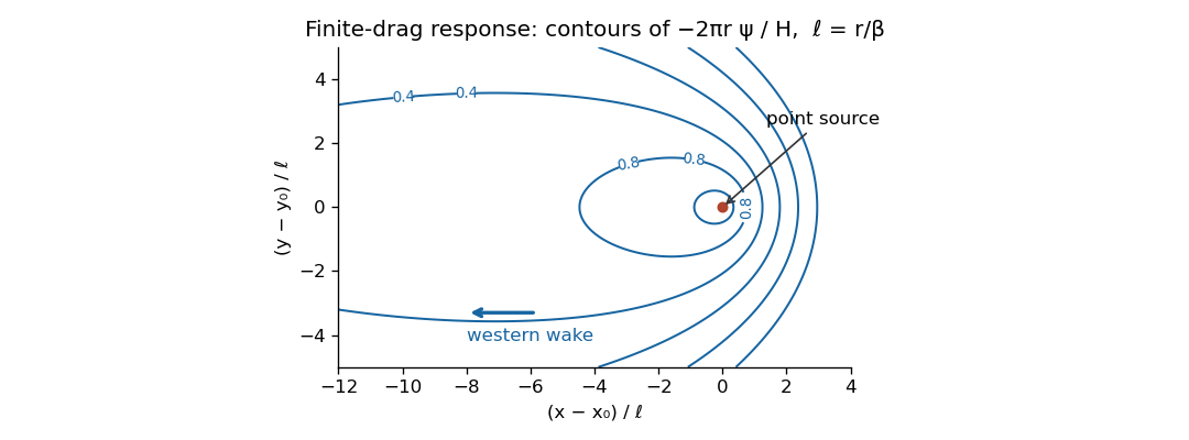
Near the source the logarithmic singularity produces almost circular contours. At distances large compared with $\ell =r/\beta$, $K_0(aR)\sim \sqrt{\pi /(2aR)}{e}^{-aR}$, so the response is proportional to $e^{-a(R+X)}/\sqrt{R}$. It decays exponentially eastward, but only algebraically on the western axis; its broad western wake has transverse width of order $\sqrt{\ell |X|}$. Contours are stretched westward, with closed finite-level contours around the source and sharper eastern gradients. Larger drag broadens the scale $\ell$ and makes any fixed nearby view more nearly circular. For $r=0$ the elliptic smoothing disappears; for $\beta =0$ the infinite-plane response is logarithmic up to a gauge and cannot be fixed by a zero-at-infinity condition.

Write the parabolic depth as $H(x)=ax(L_x-x)$ with $a>0$, and use $f=f_0+\beta y$, $\beta >0$. The topographic potential-vorticity pseudovelocity isIt is westward everywhere in the interior. In the Northern Hemisphere it is also southward on the western slope and northward on the eastern slope. Its characteristics are the background potential vorticity contourswhich bend towards the south on approaching either shallow side. Along these characteristics forcing accumulates into a transport response and drag spreads it across neighboring characteristics. The actual current follows contours of $\psi$, not contours of this pseudovelocity in a forced region.

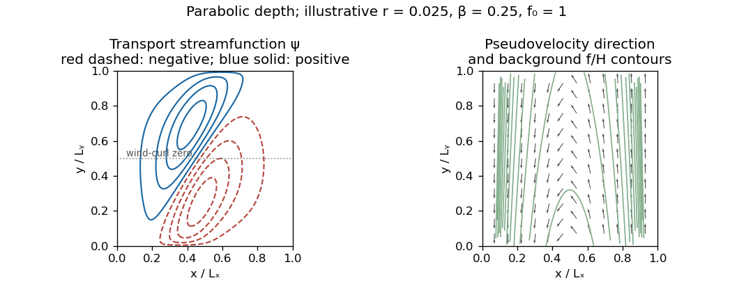
The sketch uses an explicit illustrative positive drag, a single connected impermeable boundary with $\psi =0$, $H=4x(1-x)$, and $f=1+0.25y$ in normalized coordinates, with small forcing amplitude $F_0=10^{-3}$; linearity makes its value affect amplitudes rather than contour shapes. Solid and dashed contours distinguish the two signs of $\psi$; arrows indicate the pseudovelocity, not the real current. The positive lower-half wind curl tends to drive cyclonic circulation and the negative upper-half wind curl anticyclonic circulation; topographic steering bends the gyres, so their dividing contour need not coincide with the forcing's zero line. The plot is an example, not a uniquely specified circulation: the question supplies neither a drag magnitude nor full boundary data.

The westward propagation of transport information explains the connection with western boundary currents: a broad wind-driven interior generally needs a narrow western return region to satisfy the impermeable boundary condition. For constant depth the characteristic direction is purely westward and the Stommel boundary layer width is $r/\beta$ for this drag normalization. Here strong depth gradients also steer the return along slopes and can make topographic boundary currents important; a conventional flat-bottom western-current profile does not follow unchanged. The equation becomes singular where $H=0$. The drawn shore limits impose zero transport; a physically resolved shoreline would need a positive-depth cutoff or a separate near-shore model, and the small-Rossby number approximation need not remain uniform there.