Use an upward vertical coordinate , constant mass density , and a positive Coriolis parameter ; the square-root formulas below assume the Northern Hemisphere. For a slab of thickness , the net force per unit horizontal area is . Dividing by its mass and including the Coriolis acceleration givesHere are the vertical shear stress components of the viscous stress tensor, so their boundary values require a signed traction convention. Linearization removes advective acceleration. Decompose the horizontal velocity into an exterior pressure response and an Ekman layer correction. On an f-plane these satisfyandThe exterior pressure response is in geostrophic balance when steady. For a surface Ekman layer with negligible stress at its base, its Ekman transport isIntegrating the continuity equation and imposing zero vertical boundary-layer velocity at the surface gives . Thus the base velocity, positive upward, isThe PDF prints the opposite sign. Its negative formula is correct for a velocity defined positive downward, but its stated momentum equations with use the upward-coordinate shear convention above. This sign must be accounted for when interpreting the subsequent pumping equation.
For constant kinematic viscosity, write and . The steady Ekman layer equation is . Taking the surface at and the ocean below it, the bounded surface Ekman layer solution isThe total velocity is . Prescribed wind stress determines the coefficient of this Ekman layer correction; it does not determine a relation between the wind and the independent pressure-driven velocity. An additional boundary condition is necessary for a laminar Ekman boundary stress law in terms of .
The two printed laminar stress formulas and the positive pressure-Laplacian pumping formula are instead the standard Bottom Ekman layer relations. To derive them consistently, put a stationary no-slip boundary condition at , with water at . ThenConsequentlyThese are shear stress values; the actual bottom traction on the fluid has the opposite sign. Integrating this Bottom Ekman layer gives and . Since the exterior geostrophic flow is horizontally nondivergent, the upward velocity above the bottom is . Using , yieldsThis recovers the requested magnitude and pressure dependence with a consistent bottom interpretation. The surface version would require its own specified boundary velocity and corresponding signs.
For Ekman spin-down in a shallow-water layer, let , , and . Upward bottom pumping enters the exterior linearized shallow water equations through . Taking the curl of their momentum equations gives , henceSlow geostrophic balance gives and . Therefore the intended damping equation isThe slow-adjustment assumption is , not the printed . The printed negative pumping term in continuity can alternatively describe downward extraction at the upper boundary, but it cannot be combined unchanged with the upward bottom pumping just derived. A literal use of the positive printed and negative continuity source would reverse the damping sign and produce growth.
For a Fourier mode with , substitution givesFor scales small compared with the Rossby deformation radius, and , independent of wavenumber. For scales large compared with the Rossby deformation radius, the equation becomes , whereThe zero wavenumber mode does not decay. A thin Ekman layer, , makes , so the derived decay time satisfies the corrected slow-time assumption.
The vertical component is times the first-order anomaly in shallow-water potential vorticity about rest:Thus records the combination of relative vorticity and column stretching that is conserved by the unforced linearized shallow water equations. Indeed their curl and continuity equation give . It is the persistent forcing of the balanced component during geostrophic adjustment, while inertia-gravity waves carry away the unbalanced component.
Initially . In the final geostrophic flow, , , and . Conservation of the linearized shallow-water potential vorticity therefore givesBoundedness on both sides and continuity of at the origin determine the constants:The solution is the locally attained balanced state after outgoing inertia-gravity waves have departed; the full inviscid system need not lose its globally conserved wave energy. The signed volume flux in the direction is
For double Kelvin-wave adjustment at a depth step, put and use on the corresponding side of the step. The PDF's far-field wording must mean , rather than for every . In the exponentially trapped outer response, cross-step geostrophic balance gives, at ,To retain the propagation of this slowly varying trapped disturbance, the along-step acceleration in must also be retained. It supplies the small cross-step ageostrophic flow. Thus the two cross-step volume fluxes areHere as a distributional derivative. Equating the fluxes and dividing by givesThe printed forcing is missing a factor of two. It cannot follow from the printed sign-function surface profile with the usual Dirac delta distribution normalization. Pure geostrophic balance in both horizontal directions would also omit and could not determine the wave evolution.
The method of characteristics with zero initial amplitude gives the corrected weak solutionBehind the eastward front, , the surface elevation at the step becomes , matching the upstream side. All the original cross-step transport is diverted into flow along the step once the wave has passed a fixed location: there, with opposing along-step velocities above and below the step. This is the complete barrier in the adjusted region, and in the long-time limit at every fixed . At finite time a front still carries cross-step flux: the formulas above give . The discontinuous outer representation does not resolve the short-scale fast adjustment at either front.
For completeness, solving the equation literally as printed instead gives . Its amplitude is half that required; retains a jump at the origin after passage, so that literal equation does not imply complete blocking. The corrected equation and the literal printed equation are distinguished rather than asserting an inconsistent barrier result.
Assume inviscid, unforced evolution, so shallow-water potential vorticity is conserved. If a column has initial depth and relative vorticity , moving to at fixed Coriolis parameter givesIts absolute vorticity is amplified by vortex stretching. A column initially without relative vorticity develops cyclonic spin: positive in the Northern Hemisphere and negative in the Southern Hemisphere. More generally the increase is in the direction of its original absolute vorticity, not necessarily the direction of if the initial spin is unusually strong.
Conservation of shallow-water potential vorticity with fixed relative vorticity givesFor ordinary planetary-vorticity-dominated columns, moving towards the equator decreases the magnitude of absolute vorticity, so the column must become shallower and spread horizontally. This is the compression counterpart of vortex stretching. For , the depth ratio is , in either hemisphere before reaching the equator. The displayed general formula is essential if the fixed relative vorticity is large: the sign of the depth change then depends on the original absolute vorticity, and conservation cannot continue through zero absolute vorticity with positive finite depth and nonzero conserved potential vorticity.
Use a one-layer, hydrostatic, homogeneous fluid with reference depth , no forcing or friction, small Rossby number , slow evolution, and leading geostrophic balance. For the beta plane, take ; the relative free-surface displacement is also small, , with the Rossby deformation radius retained at the chosen horizontal scale. This excludes the equatorial limit. If a bottom elevation is included, additionally require and stationary topography. Set for a flat bottom.
The quasi-geostrophic streamfunction satisfies , , , so relative vorticity is . Expanding the shallow-water potential vorticity using actual depth givesConsequently the depth-scaled anomaly, the shallow-water quasi-geostrophic potential vorticity, isThe leading material derivative uses the geostrophic flow. Define ; then conservation yields . The term represents free-surface stretching, the variation of planetary rotation, and topographic stretching. Under a rigid lid or at scales much smaller than the Rossby deformation radius, the free-surface term is absent or negligible and the flat-bottom Barotropic Rossby wave model has .
For a zonal basic geostrophic flow , take and write . The flat-bottom shallow-water quasi-geostrophic potential vorticity gradient of the basic state isLinearizing its material conservation gives the Rossby-wave equation for a sheared zonal current,For a general nonuniform jet, a global two-dimensional plane wave is not an exact normal mode: the coefficients depend on . The exact zonal normal mode problem, , iswith appropriate transverse boundary or radiation conditions. If the jet varies slowly compared with a wavelength, a local plane wave freezes these coefficients at . Its local dispersion relation isIn the nondivergent Barotropic Rossby wave model under a rigid-lid approximation, this becomes . It is exact for uniform and otherwise a local relation. Retaining the free-surface term also requires retaining the basic surface slope in ; simply adding to the denominator while dropping from the numerator would describe a different prescribed-background model.
Take , a uniform eastward , and the nondivergent Barotropic Rossby wave model. Its dispersion relation is . A stationary wave with hasThe directional component wavelengths are and when nonzero. Differentiating the full dispersion relation before imposing stationarity gives its ground-frame group velocity:Writing , shows . Therefore the stationary Rossby-wave ray envelope at time , for wave packets emitted from a localized mountain throughout , is the diskThe circle is the front of the earliest emissions; later emissions fill ray segments back to the source. The sketch represents the geometrical wave packet envelope, not compact support of the full balanced near field. All propagating wave packet energy lies downstream in this model.
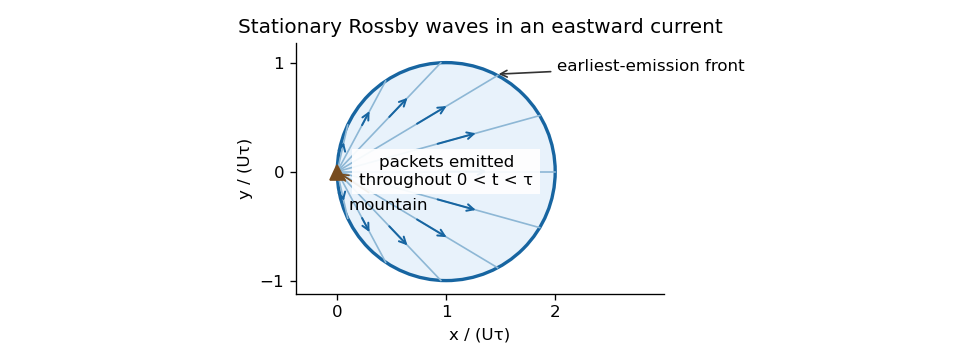
Downstream ray envelope of stationary barotropic Rossby waves emitted by a mountain between zero and the observation time
. Details. 
If the finite-depth free-surface model of the preceding part is retained consistently, its basic surface slope adds to the potential-vorticity gradient. Stationarity still gives and the same wavelength, but the group velocity is reduced by ; the disk center and radius become . This tends to the plotted nondivergent result as .
A westward wind has no nontrivial stationary propagating planetary Rossby-wave train in this model: would require . Its advective phase motion and intrinsic westward Rossby wave phase motion cannot cancel. A local forced, evanescent response and time-dependent disturbances can still occur. The degenerate limit is not a propagating wave train from an isolated mountain.
For steady depth and no sources of fluid mass, the continuity equation gives . In a simply connected region this defines an ocean transport streamfunction:A multiply connected basin additionally needs its circulation or boundary-constant data. Taking the vertical curl of gives the exact relative vorticity from a variable-depth transport streamfunction relationNo small-depth-variation expansion has been made. No normal flow at a basin wall means that is constant along that connected wall.
Let . At sufficiently small Rossby number, retain advection of this full background shallow-water potential vorticity while dropping the higher-order advection of . For uniform-depth Sverdrup balance, this also requires relative-vorticity advection to be small against planetary-vorticity advection; small Rossby number alone does not guarantee this when is very small. Multiplying the resulting steady potential vorticity equation by givesDefine the topographic potential-vorticity pseudovelocityIts sign is important: it is opposite to the coefficient vector on the left of the preceding equation. Substituting the ocean transport streamfunction expression for relative vorticity yieldsThe pseudovelocity follows contours of and is not the fluid velocity; its units are inverse length squared per time because is a transport streamfunction. If , the ocean transport streamfunction is constant along each connected background potential vorticity contour. Locally, at regular points,with arbitrary differentiable . Different disconnected components of a level set may carry different functions until boundary conditions identify them. If is constant over an open region, the leading equation gives no restriction there; critical points similarly require regularity and global matching rather than division by a vanishing gradient.
For uniform depth on a beta plane, . With weak bottom drag the equation reduces to Sverdrup balance,Restore a dimensional forcing amplitude ; the printed unit-amplitude forcing means in the chosen units. The general interior ocean transport streamfunction isTaking on a straight eastern boundary sets ; without a zonal boundary condition the function remains arbitrary. ThenThe Sverdrup balance interior cannot satisfy both zonal-wall conditions; a western boundary current supplies the return circulation.
For basin scales , use , , and . The ratio of drag to Sverdrup balance terms is of orderThis criterion applies away from boundary layers and zeros of the leading forcing, with positive , , and the beta plane and small-Rossby number assumptions. For an approximately square basin it is . Neglect of nonlinear relative-vorticity advection further requires for comparable velocity and length scales. Thus weak drag relative to the balance, rather than just a small absolute , is the appropriate condition.
Put , and take . The constant-depth ocean transport streamfunction equation isIt is a steady advection-diffusion equation for the transport response, with westward pseudovelocity. For an unbounded domain the point-forced Sverdrup–drag Green function can make its contours precise. Set and . Thenwhere is the Modified Bessel function of the second kind. This optional explicit expression is used only to produce the requested sketch; no weak-drag assumption is imposed.
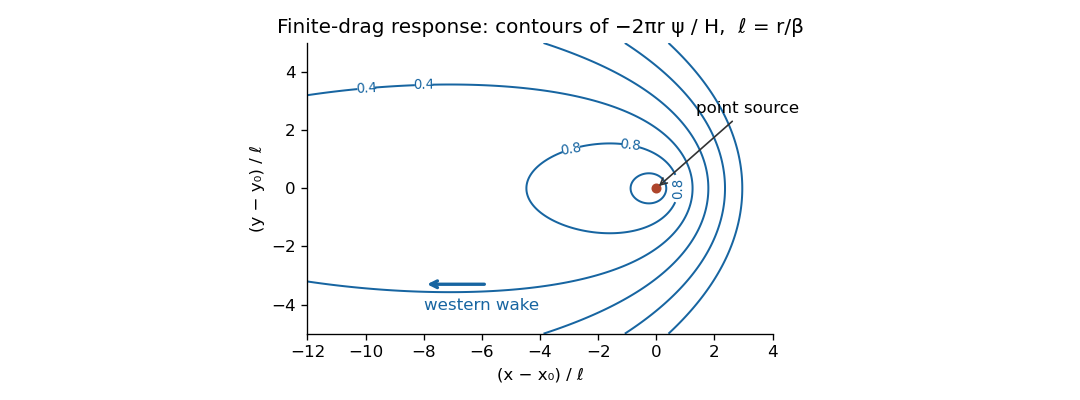
Streamfunction contours around a point wind-curl source with finite bottom drag, showing a long western wake and a short eastern response
. Details. 
Near the source the logarithmic singularity produces almost circular contours. At distances large compared with , , so the response is proportional to . It decays exponentially eastward, but only algebraically on the western axis; its broad western wake has transverse width of order . Contours are stretched westward, with closed finite-level contours around the source and sharper eastern gradients. Larger drag broadens the scale and makes any fixed nearby view more nearly circular. For the elliptic smoothing disappears; for the infinite-plane response is logarithmic up to a gauge and cannot be fixed by a zero-at-infinity condition.
Write the parabolic depth as with , and use , . The topographic potential-vorticity pseudovelocity isIt is westward everywhere in the interior. In the Northern Hemisphere it is also southward on the western slope and northward on the eastern slope. Its characteristics are the background potential vorticity contourswhich bend towards the south on approaching either shallow side. Along these characteristics forcing accumulates into a transport response and drag spreads it across neighboring characteristics. The actual current follows contours of , not contours of this pseudovelocity in a forced region.
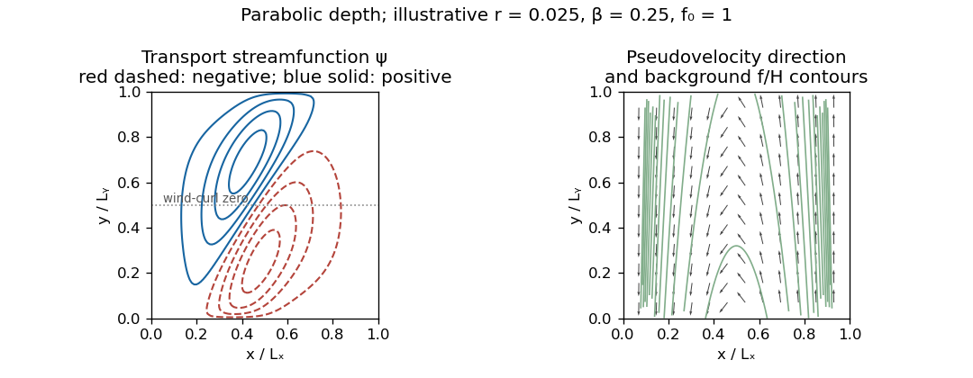
Illustrative wind-driven streamfunction contours and westward topographic pseudovelocity in a basin with parabolic depth and no normal boundary transport
. Details. 
The sketch uses an explicit illustrative positive drag, a single connected impermeable boundary with , , and in normalized coordinates, with small forcing amplitude ; linearity makes its value affect amplitudes rather than contour shapes. Solid and dashed contours distinguish the two signs of ; arrows indicate the pseudovelocity, not the real current. The positive lower-half wind curl tends to drive cyclonic circulation and the negative upper-half wind curl anticyclonic circulation; topographic steering bends the gyres, so their dividing contour need not coincide with the forcing's zero line. The plot is an example, not a uniquely specified circulation: the question supplies neither a drag magnitude nor full boundary data.
The westward propagation of transport information explains the connection with western boundary currents: a broad wind-driven interior generally needs a narrow western return region to satisfy the impermeable boundary condition. For constant depth the characteristic direction is purely westward and the Stommel boundary layer width is for this drag normalization. Here strong depth gradients also steer the return along slopes and can make topographic boundary currents important; a conventional flat-bottom western-current profile does not follow unchanged. The equation becomes singular where . The drawn shore limits impose zero transport; a physically resolved shoreline would need a positive-depth cutoff or a separate near-shore model, and the small-Rossby number approximation need not remain uniform there.
Articles by others on the same topic
There are currently no matching articles.