The initial table of content was limited to the first level because it is larger than 1000 articles. There are 2764 articles in total. Expand a branch to load its children.
The quadratic formula givesso both roots of a polynomial have real part . Writing , the complex exponential function satisfies , and hence its modulus is . ThereforeIntersecting this condition with the allowed parameter interval gives the answer for either root:The endpoint is included: the repeated root of a polynomial is , whose exponential has modulus .
Write the complex number as . Since , the modulus of the complex exponential givesThis equals one precisely when . The quadratic formula shows that the imaginary part of either root is . Consequently the roots are real exactly at the two endpoints:Both endpoints satisfy the condition. The repeated roots are respectively and ; their multiples by have exponentials on the unit circle.
Using the exponential definition of the hyperbolic cosine and the complex exponential function,ThusFor real , the hyperbolic sine vanishes only at . Also , so the only zero of sine available to is . The product therefore vanishes exactly when or :There are three possible parameter values. At the roots are and is real; at the roots themselves are real.
A counterclockwise planar rotation matrix has the formTo recover this form from preservation of the Euclidean norm, let be the columns of . Applying the norm condition to the two coordinate unit vectors gives . Applying it to their sum givesso . The columns are an orthonormal basis, and : is an orthogonal matrix.
Write . There are two perpendicular unit vectors available for , namely . The first gives determinant , the second . The positive determinant hypothesis selects the first. A norm-preserving planar map with positive determinant is a rotation.
For the commutation condition, writeDirect matrix multiplication givesEquality forces and , so, with and ,If , take and . Otherwise set and choose , . ThenThis describes the centralizer of a planar quarter-turn. Its nonzero elements act as a rotation followed by a uniform scaling, just as multiplication by a nonzero complex number does.
A sequence is a convergent sequence with limit ifThe index may depend on , but must work for every later term.
Fix . Choose such that for , and putThis is a fixed finite number. For , the triangle inequality givesChoose sufficiently large that as well. The error is then less than , provingTaking successive arithmetic averages preserves the limit. This is the Cesaro theorem for convergent sequences: any troublesome initial terms contribute only a fixed numerator divided by .
Every counted point has integer coordinates and lies in the square , while the origin is always counted. HenceNo precise circle-area estimate is needed; this elementary bound controls the growth of the power series coefficients.
The comparison test for series states that if , convergence of implies convergence of . Equivalently, divergence of the smaller nonnegative series forces divergence of the larger one.
For ,For , the ratio of successive terms on the right tends to , so the ratio test and the comparison test for series show absolute convergence. The case is immediate.
If , then , so the terms do not tend to zero. The term test for divergence therefore rules out convergence, including every point on the boundary . Thus the radius of convergence isThe series converges exactly in the open unit disc. This is an example of polynomial coefficient growth with unit power-series radius: the lattice-count bound is polynomial rather than exponential.
Use suffix notation with indices ranging from to , and sum over repeated indices. By the component definitions of the dot product and cross product,The Levi-Civita symbol is unchanged by a cyclic permutation of its three indices: the cycle is two transpositions and hence has positive sign. Thus . Commuting the scalar components givesTherefore the scalar triple product obeysCyclically moving the vectors preserves the scalar triple product; interchanging just two reverses its sign.
The two displacement vectors and lie in the required plane. Because the three points are non-collinear, their cross productis nonzero and is a normal vector to that plane. A point with position vector lies in the plane exactly whenExpanding the cross product givesThe terms and vanish, so the equation of a plane through three points becomesNon-collinearity is important: it ensures this is a genuine plane equation with nonzero normal, rather than the vacuous equality .
For the specified coordinates,Their sum is , with Euclidean norm . Consequently either orientation of the unit normal is valid:As a check, the scalar triple product is , so the plane equation simplifies to , which all three supplied points satisfy. The normal direction is .
The chosen unit normal points toward the plane from the origin, so the plane equation isTo locate the circle centre, project onto this plane. PutThen , so lies in the plane. For any other point of the plane, is perpendicular to . The Pythagorean theorem therefore givesRestricting the sphere equation to the plane consequently gives a circle centred at . Thus , proving that the displacement of its centre is purely normal:The same Pythagorean theorem gives , and henceThe sign of is fixed by which side of the plane contains ; and alone determine only its magnitude. Substituting the signed offset yields the sphere-plane intersection radiusA genuine circle requires ; equality gives tangency and , while a larger distance gives no intersection. The signed distance from a point to a plane in the direction is ; the ordinary distance from a point to a plane is its absolute value.
For the reality of the eigenvalues, one may initially allow a nonzero complex eigenvector with . Since is real symmetric, it is a Hermitian matrix, andis real: the numerator equals its own complex conjugate and the denominator is positive. Once is real, a nonzero real or imaginary part of supplies a real eigenvector. We work with the real unit eigenvectors of the problem.
For two such eigenvectors, symmetry givesDistinct eigenvalues therefore give zero dot product. Together with the prescribed unit lengths,These vectors form an orthonormal basis of .
Expand a real unit vector as . Then , and its Rayleigh quotient isMoreover,Every coefficient on the right is strictly positive, so equality forces for . Equality occurs precisely along the top eigendirection:
To obtain a unit vector in using just , let and denote their first coordinates. If , takeThen and . Hence has first coordinate zero and unit length. If , simply take . In either case the Rayleigh quotient of the constructed vector isThe continuous quadratic form attains its maximum on the compact space , so
For , deletion of the first row and column gives , while . The spectral theorem for real symmetric matrices applied to identifies its largest eigenvalue with this maximum:Combining the upper bound for every unit vector with the constructed lower bound provesThis is largest-eigenvalue interlacing for a principal submatrix: restricting a quadratic form to a coordinate hyperplane cannot exceed its old maximum, but leaves some direction in the span of the top two eigenvectors.
A matrix is a diagonalizable matrix if there is an invertible matrix for which is diagonal. Its columns then form a basis of eigenvectors, and the diagonal entries are their corresponding eigenvalues.
Here the given eigenvectors form an orthonormal basis. Put them into the columns of :Define . Its entries areThis proves the claimed diagonalization of a matrix, rather than merely guessing it:The trace follows directly from this factorization:because each column of has unit length. Trace is the sum of the eigenvalues, with multiplicity.
For the particular matrix, . If , every contributes one and contributes zero. If , precisely and contribute zero; the other terms contribute one. ThusApplying this identity to a nonzero eigenvector givesEvery eigenvalue is therefore or .
If is the multiplicity of , the trace formula for a diagonalizable matrix and the zero diagonal giveso . Up to ordering, the required diagonal form isFor this means just . For , the eigendirections are also transparent: the all-ones vector has eigenvalue , and the -dimensional subspace whose coordinate sum is zero has eigenvalue , since . The spectrum consists of one collective mode and zero-sum modes.
Adding the three equations for gives the necessary solvability condition . Conversely, subtraction of the first two and use of the third forceIf , these values also satisfy the first two equations: for example,The analogous calculation gives . Thus existence and uniqueness hold exactly under the stated compatibility condition:
For the three-variable system the matrix and data vector arePerform Gaussian elimination on the augmented matrix. The operations and giveEach operation is an invertible row scaling followed by a row addition, so the solution set is preserved. Next givesBack substitution now yieldsand thenAll three pivots are nonzero. Thus the solution exists uniquely for every , the matrix rank is , and the kernel of a linear map represented by is . The general rank-nullity theorem for a matrix with columns ishere .
Finally, reverse the viewpoint and regard as prescribed. The necessary and sufficient condition already proved applies with , , . Their sum is . Consequently can be recovered exactly whenWhen this holds, their unique values are and . The allowable triples form an affine plane, not all of .
A complex square matrix is a unitary matrix when , equivalently . Here denotes the adjoint matrix, the conjugate transpose. Such a matrix preserves the standard complex inner product and its Euclidean norm.
A real symmetric matrix is a Hermitian matrix, so . For arbitrary complex ,The imaginary cross terms cancel because is Hermitian. Reversing the signs gives the same identity:In particular, implies , so has zero kernel of a linear map. It is a square matrix, and the rank-nullity theorem therefore makes it invertible. The same argument proves invertibility of .
The proposed matrixis consequently well-defined. For any , put . The two norm identities show directly thatTo verify the unitary matrix identity explicitly, take adjoints:The two shifts commute, because both are polynomials in . HenceThusThe imaginary shifts are invertible, and their equal norm changes cancel in the quotient. This is the Cayley transform of a Hermitian matrix in the convention.
The Bolzano-Weierstrass theorem states that every bounded sequence of real numbers has a convergent subsequence. We first use it to show that a continuous function on is bounded above. Otherwise, choose with . A convergent subsequence exists, with because the interval is closed. Continuity would give , contradicting .
Let , which is finite. By the definition of supremum, there are with . Another application of the Bolzano-Weierstrass theorem gives a subsequence . By continuity,Thus the supremum is actually attained:This proves the maximum part of the extreme value theorem from sequential compactness rather than assuming it.
Now suppose on . Applying the mean value theorem to shows that is strictly decreasing. At a local maximum of a differentiable function, the left difference quotients are nonnegative and the right difference quotients are nonpositive; existence of the derivative forces . A strictly decreasing function has at most one zero. ThereforeIf that zero exists, is positive to its left and negative to its right, so the local maximum is also a global maximum.
For the uniform bound by , defineIts derivative is , so is strictly decreasing by the mean value theorem. Comparing with givesBecause , this makes negative at sufficiently large positive and positive at sufficiently large negative . The function is continuous, since it is differentiable; the intermediate value theorem supplies a zero between such points. Its strict decrease makes this zero unique. Again using the mean value theorem for , the derivative signs imply that increases up to and decreases after :This illustrates uniform negative curvature and global maximization.
Merely requiring does not force existence. TakeThen and , but is strictly increasing, approaches as , and never equals . The answer to the final question is no, even for a function bounded above:The stronger uniform curvature assumption prevents this behaviour. Here at the end where the supremum is approached, so no uniform negative bound of that kind is available.
The Rolle theorem states that if a real function is continuous on , differentiable on , and has equal endpoint values, then its derivative vanishes somewhere in . Order the distinct real roots as . The theorem gives a root of in each interval . These intervals are disjoint, so the obtained roots are distinct:
We prove the requested bound for positive roots of a polynomial by mathematical induction on the number of nonzero terms. In fact, the proof also works with roots counted according to their multiplicity. Write for the number of sign changes and for the positive-root count.
A one-term polynomial has no positive roots and no sign changes. For the induction step, factor out the smallest power of :For this factor is nonzero, so , including multiplicities, and . Differentiation removes exactly the constant term:The exponents remain strictly increasing, and the positive multipliers do not change coefficient signs. The induction hypothesis therefore gives
First suppose . Removing removes exactly one sign change, so . If has positive roots of multiplicities , its derivative has multiplicity at and, by the Rolle theorem, an additional root between each pair. Thus the Rolle root count with multiplicities giveswhen there is a positive root. ConsequentlyIf there is no positive root, the desired bound is automatic.
Now suppose , so . Again the zero-root case is immediate. Otherwise, multiplying by if necessary lets us assume and without changing roots or sign changes. For sufficiently small ,since and the lowest-power term of has positive coefficient. Choose such a point before the first positive root . The mean value theorem on gives a point withBut . The intermediate value theorem applied to the polynomial therefore gives an extra root in , before . It is distinct from the roots at and those between consecutive roots. HenceBoth sign cases complete the induction:An initial sign change allows one extra positive root; without that sign change, the derivative must already turn before the first positive root. This is the upper-bound part of the Descartes rule of signs. The multiplicity claim used above follows by differentiating with : the derivative has a factor and its remaining factor is nonzero at .
The two preliminary sequence limit laws follow directly from the triangle inequality. For the sum, choose indices so that and beyond their respective cutoffs. Beyond the larger cutoff,Thus
For the reciprocal, convergence to nonzero gives eventually. The reverse triangle inequality then gives , and consequentlyChoosing the eventual error smaller than both and provesThe nonzero limit gives the denominator a positive lower bound; nonzero individual terms alone would not do so. The assumption ensures the reciprocal sequence is defined even before this eventual bound applies.
Use rationalization of a square-root difference to avoid subtracting two large, nearly equal quantities:Since and the square root is continuous at , the denominator tends to . The reciprocal limit law established above is applicable because this limit is nonzero. HenceThe limit is one half; rationalization exposes the finite difference hidden by cancellation.
Rationalize the numerator of the summand:For every we have , and thereforeThe harmonic series diverges, so the comparison test for series makes the given positive-term series diverge as well:For completeness, divergence of the harmonic series follows by grouping the terms with : each such block contributes at least . The same rationalization also shows that times the summand tends to . The summands tend to zero, but their harmonic-size tail prevents convergence.
The stated bound is Lipschitz continuity with constant . For every and every , taking ensures whenever . The same works at every point, so is both continuous and uniformly continuous.
For an integer , partition into equal intervals and define a step functionAt the remaining endpoint set , so the final interval may be taken closed on the right. The Lipschitz bound givesChoosing proves the requested uniform step approximation on a compact interval:A sufficiently fine partition gives a piecewise constant approximation uniformly over the whole interval.
The continuous function and every finite step function are Riemann integrable. Put . Integrating each constant piece explicitly givesSince the sine differences have absolute value at most , the triangle inequality and uniform approximation giveTo prove convergence, fix and first choose with . With this held fixed, the finite number is independent of , so the second term is also less than for sufficiently large . ThereforeFirst make the approximation error small, then let the oscillation frequency grow. This is the step-function proof of the Riemann-Lebesgue lemma; it does not require assuming that a Lipschitz function has an everywhere-defined derivative.
The characteristic polynomial of this second-order linear differential equation factors as . Its two distinct roots give the general solution . Boundedness as forces , and the initial condition gives .
The required solution is
Collecting the shifted terms gives a second-order difference equation with coefficients , and . Substitute to obtain its characteristic equation of a linear recurrence:For real , the roots and general solution areIn the small-step regime, indeed for , the polynomial is positive at , negative at and positive for sufficiently large positive . Thus . The bounded solution of a second-order constant-coefficient recurrence discards the growing root, and fixes its remaining coefficient:The Taylor series establishes the displayed approximation to the root. Raising that approximation to the th power is a leading approximation, rather than a uniform relative approximation for arbitrarily large : its relative error is controlled when is small. For completeness, the degenerate values give when , and when .
Divide the second-order difference equation by and set . The first quotient is a central finite difference approximation to ; the quotient approximates . Their Taylor series errors are for a sufficiently smooth function. This is therefore a finite difference method for the second-order linear differential equation in part (a).
At a fixed , take with integral. Since , the exact bounded discrete solution satisfiesLikewise . The decay selected by boundedness in the linear recurrence relation becomes exactly the decay selected by boundedness in the ordinary differential equation.
Start from . Differentiation under the integral sign givesThis interchange is justified locally around any by the dominated convergence theorem: the differentiated integrands are bounded by an integrable polynomial times . Successive derivatives of giveThis is also the integer case of the Gamma function integral after scaling the integration variable.
Use the inverse change of variables and . The chain rule gives the differential operatorsThe mixed partial derivatives cancel, assuming the twice continuously differentiable solution appropriate here. Consequently .
The transformed equation isThe factors of belong to the inverse Jacobian matrix; using the forward transformation instead would give an incorrect factor.
The independent and identically distributed random variables have a continuous probability distribution, so any tie has probability zero. Their joint probability density is unchanged by a permutation of their indices: this is order symmetry of independent random variables. The strict orderings are disjoint and exhaust the sample space apart from the zero-probability ties. Each ordering therefore has the same probability, and their probabilities sum to one.
The probability is
The moment-generating function of a random variable is , at the real values of for which that expectation is finite. For a standard normal distribution variable , combining the exponentials in its probability density function yieldsThe last equality follows by scaling the Gaussian integral. The variables are independent random variables, so the expectation of their product factorizes. ThereforeThis is the moment-generating function of a chi-squared distribution with degrees of freedom. For positive the defining integral diverges at and above .
Away from the impulse, the harmonic oscillator equation has a homogeneous solution. Before , the initial conditions select . The jump condition for an impulse requires continuity of and a unit jump in : a jump in would produce a derivative of the Dirac delta distribution, which is absent from the forcing, while integrating through the impulse gives .
Just before the impulse, and . Just afterwards, and , so uniqueness for the harmonic oscillator equation makes the subsequent solution identically zero. Equivalently the causal response is , with the Heaviside step function, and it cancels the original oscillation.
The solution isThe impulse cancellation of a harmonic oscillator produces a continuous graph with a corner at , followed by a horizontal zero line.
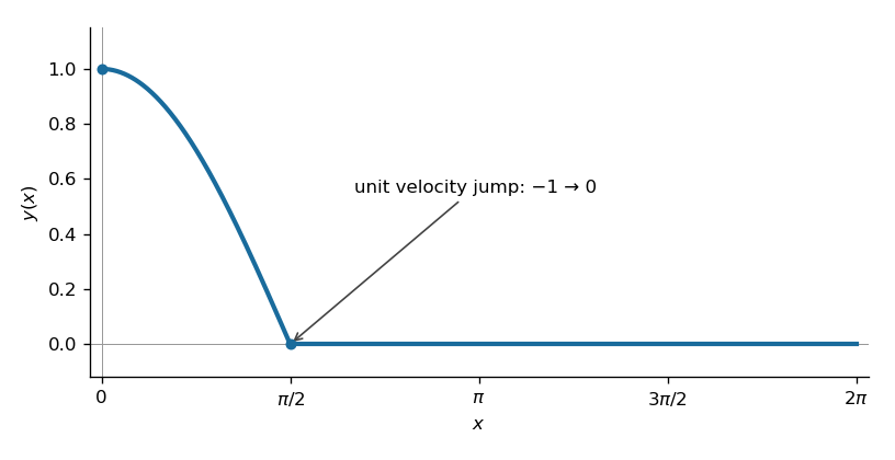
An impulse cancels the oscillator at zero displacement
. With a positive cooling rate , Newton's law of cooling gives . The temperature excess satisfies the first-order linear differential equation . Applying the initial condition to its exponential decay solution givesThe temperature approaches the ambient value , rather than zero. The intended cooling situation has and .
At the first half-temperature time, the solution of Newton's law of cooling givesSince , this time is positive and finite. The instantaneous temperature increase supplies the new initial condition . Restart the same first-order linear differential equation at :This is Newton cooling with an instantaneous temperature jump. The time translation in the exponential decay is essential: its prefactor is the excess immediately after the jump.
Each smooth segment follows Newton's law of cooling: and . Thus the graph decreases and is convex on both sides of . It starts at , falls to , jumps upward by , and then decreases asymptotically to .
The right-hand limit at the jump is above the original temperature, because implies . The vertical dotted segment in the sketch denotes an instantaneous jump, not a continuous evolution through intermediate temperatures. The example uses , ; its qualitative shape holds for all the stipulated parameters.
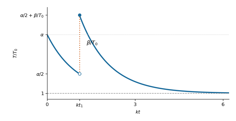
Cooling interrupted by an instantaneous temperature increase
. Impose the target temperature on the post-jump exponential decay:Solving for the jump and eliminating using givesThis is the unique required temperature increase, and it satisfies the stipulated lower bound. Indeed impliesThus no additional restriction on the prescribed time is needed.
For the stated order of the two solutions, define their Wronskian byTaking a derivative cancels the two mixed products: . Substituting the second-order linear differential equation for each second derivative cancels the terms and leavesThis is the Abel identity. On an interval with continuous coefficients, linear independence means ; hence the Wronskian never vanishes anywhere on that interval.
The defining Wronskian identity gives the first-order linear differential equationWork first on an interval where . Dividing by recognizes a derivative:This is reduction of order. Choose the nonzero Wronskian from the Abel identity to obtain linear independence. The constant only adds a multiple of . If has zeros, this quotient formula is local; the resulting solution can be continued across ordinary zeros using the original second-order linear differential equation.
For real parameters, work on so arbitrary real powers are unambiguous. Taking derivatives givesThe residual after substitution isWhen , ranges over . Evaluating at the zeros of the cosine first forces the sine coefficient to vanish; then the cosine coefficient vanishes identically. If , the nonzero constant cannot satisfy the equation. Thus the necessary and sufficient conditions areUnder these conditions the normalized coefficient is . The Abel identity gives . Choose and apply reduction of order on an interval where :The substitution evaluates the integral. After continuation across the cosine zeros,This is a power substitution for an oscillatory second-order equation: in the variable , the equation reduces to the harmonic oscillator equation.
Classification and characteristic exponents. For a normalized second-order linear differential equation, an ordinary point at zero means and are real analytic functions there. A regular singular point is a singular point where and nevertheless extend as real analytic functions to zero. Write and . The lowest-power coefficient in the Frobenius method gives the indicial equationIts roots are the characteristic exponents at a regular singular point. If their difference is not an integer, there are two linearly independent solutions , with real analytic and . For distinct real roots with integer difference, a solution for the larger root exists, and a second has the form ; the logarithmic coefficient can vanish. For a repeated root, the second solution has the form after normalization. This is a Logarithmic Frobenius solution. Complex conjugate roots give real solutions whose leading behaviour is and , with analytic-series corrections. All these descriptions are on , or on a fixed complex branch.
For the present equation, division by gives and . Therefore and are real analytic. Zero is regular singular when ; when , it is ordinary after removing the common factor . In that exceptional case the normalized equation is .
For the Frobenius method substitution, the lowest coefficient and the general linear recurrence relation areThese equations come respectively from the coefficients of and . At , the same formal exponents describe the two possible leading powers at an ordinary point, rather than singular behaviour.
For the exponent , the linear recurrence relation reduces to . The excluded nonpositive integers ensure that no denominator is zero. Normalize and iterate:The ratio test gives an infinite radius of convergence for the power series factor. Hence a solution isFor nonintegral , choose instead the exponent . Since for every positive integer , its linear recurrence relation gives . ThusThe distinct nonintegral leading exponents establish linear independence. More explicitly, by the Abel identity and the leading coefficient at zero, so the Wronskian is nonzero. The factor uses the real branch on .
For positive integral , the exponent-zero linear recurrence relation fixes for , but at its factor vanishes and leaves free. Choose and . All later coefficients then vanish by the same linear recurrence relation.
A polynomial solution of degree isFor this is the constant solution , in agreement with the ordinary point exception. The terminating Frobenius series arises because the coefficient equation at the resonant index becomes , permitting truncation rather than forcing a logarithm.
Here the indicial equation has the repeated root . The first Frobenius method solution is . Since , the Abel identity gives . Reduction of order with produceswhere the additive constant is absorbed into . In particular the logarithmic coefficient is nonzero: an additional independent real analytic solution does not exist.
The general local form isThis is the repeated-root Logarithmic Frobenius solution. On the negative real side one may use , or use a fixed logarithm branch for a complex solution.
Write the system as , with . Its characteristic polynomial is , so its eigenvalues are and . An eigenvector for is . Thus is a complex solution, and its real part and imaginary part give real solutions:Their initial vectors are and , with determinant . Consequently they are linearly independent and span the two-dimensional solution space.
The general real solution is
For a constant matrix, the matrix exponential series and its differentiated series converge uniformly on bounded time intervals, as follows by comparison with the scalar exponential in a operator norm. Termwise derivatives therefore giveHence solves the initial value problem. For this particular matrix, direct multiplication gives . Splitting the matrix exponential into its even and odd powers provesThis is the matrix exponential when the square is minus the identity. If , the general solution isThe constants in part (a) are and , which makes the two forms identical.
Set and . Their inverse change of variables is , , with domain , . The absolute Jacobian determinant of this inverse transformation isUse the independence of random variables to multiply the two original Gamma distribution densities. The change of variables formula then gives the joint probability densityFactor this into two normalized densities:The support is a product domain, and the factors are precisely a Beta distribution density and a Gamma distribution density. ThereforeThis beta-gamma independence uses the common rate ; it is a rate parameter, not the scale parameter .
For any fixed bin, each ball supplies an independent Bernoulli distribution indicator with success probability . Summing the indicator variables givesThe full occupancy vector has a multinomial distribution, the basic uniform balls-in-bins allocation. Distinct bin counts are not independent when and . To see this, write . For the same ball, if , while indicators from distinct balls are independent. Their covariance is thereforeWith no balls the counts are deterministic; with one bin there are no distinct bin pairs. These degenerate cases do not contradict the conclusion.
Express the three counts as sums of indicator variables for , and . The linearity of expectation applies even though the bin counts are dependent. The binomial distribution givesThusThe relation checks the sum of these expectations. For , use the direct deterministic occupancies, or the usual binomial convention when .
There are more bins than balls, so the pigeonhole principle forces at least one empty bin. In fact . ConsequentlyFor the expected fraction, substitute into part (b). The elementary exponential limit, obtained by taking logarithms, givesThis is the empty-bin case of the Poisson limit for occupancy fractions, with limiting mean occupancy .
Articles were limited to the first 100 out of 2764 total.
Articles by others on the same topic
There are currently no matching articles.