Past exam of the mathematics course of the University of Cambridge / 2018 / iii / Paper 141 / 3

Label the four crossings $A,B,C,D$ in top, left-middle, right-middle, bottom order. Label the bounded regions $d$ (left), $e$ (right), $a$ (upper middle), $b$ (central bigon), $c$ (lower middle), and the unbounded region $o$. The drawing preserves the crossings and the orientation of the supplied figure-eight knot diagram. Its overpassing strands are the outer-left/upper-right strand at $A$, the upper-left/lower-central strand at $B$, the upper-central/lower-right strand at $C$, and the lower-left/outer-right strand at $D$.

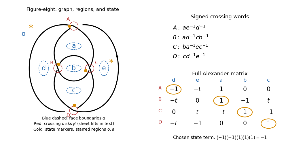
Here is the Dehn presentation Heegaard diagram specified by this drawing. Replace the underlying four-valent planar graph $G$ by a small three-dimensional regular neighborhood $N(G)$ and put $\Sigma =\partial N(G)$. Since $G$ has four vertices and eight edges, $\Sigma$ has genus $8-4+1=5$. On $\Sigma$, take the five $\alpha$ curves bordering the bounded faces, pushed slightly onto the boundary of $N(G)$. They bound a complete disk system in the complementary handlebody $S^3\setminus \mathrm{int}N(G)$; their labels are ${\alpha }_d,{\alpha }_e,{\alpha }_a,{\alpha }_b,{\alpha }_c$.

The four $\beta$ curves bound the disks dual to the four short crossing tunnels in $N(G)\setminus \mathrm{int}\nu K_8$. Lift the crossing circles shown in red onto the upper and lower sheets of $\Sigma$, routing them along the corresponding face boundaries; the crossing's overpassing strand determines the lift. Orient the $\alpha$ disk normals and the $\beta$ curves so that their signed successive intersections with the $\alpha$ curves areAt $A,D$ the missing fourth corner is the unbounded region $o$, whose generator is omitted. This sheet-lifting prescription, together with the projected graph, specifies the curves on the Heegaard surface; the red circles alone are only their local projections.

To recover the knot exterior from $\Sigma \times I$, attach five two-handles along the $\alpha$ curves on one side and cap the resulting sphere with a three-handle. On the other side attach four two-handles along the $\beta$ curves. Compressing that side leaves the boundary torus of the knot exterior, which is retained. In particular, the counts are five $\alpha$ compressions and four $\beta$ compressions, rather than two complete genus-five disk systems.

Use the region labels and curve orientations from part (a). A Dehn presentation of a knot group generator goes from the basepoint above the projection plane through its region and returns through the unbounded region. Equivalently it is dual to the correspondingly labeled $\alpha$ disk of the Heegaard diagram. A crossing relator records the signed intersections of its $\beta$ curve with these disks. Setting $o=1$ givesFor example, the overpassing strand at $A$ equates the meridian of a knot words $d$ and $a{e}^{-1}$; at $B$ it equates $a{d}^{-1}$ and $b{c}^{-1}$. The other two crossings equate $b{a}^{-1}$ with $c{e}^{-1}$ and $c{d}^{-1}$ with $e$.

Choose the region-generator direction so that $e$ is the shown meridian of a knot $\mu$. The Alexander numbering of the regions, starting from zero outside and increasing by one on crossing an oriented strand from right to left, isOne can also obtain this directly by abelianization of the relators: $a=d+e$, $c=d+e$, $b=a-d+c$, and $b-a+e-c=0$. The last two imply $d=e$, and the resulting first homology group is freely generated by $e$. Thus $H_1(X_8;\mathbb{Z})\cong \mathbb{Z}$, with no extra torsion.

Keep all four relators and all five generators, in the orders $(r_A,r_B,r_C,r_D)$ and $(d,e,a,b,c)$. Under abelianization, these generators become $(t,t,t^2,t^3,t^2)$. The Fox calculus rules areFor example, $r_B=a{d}^{-1}c{b}^{-1}$ gives the nonzero Fox derivative entries $-a{d}^{-1}$, $1$, $-a{d}^{-1}c{b}^{-1}$, $a{d}^{-1}$ in columns $d,a,b,c$, respectively. After abelianization these are $-t,1,-1,t$. The full Alexander matrix isThe Fox calculus identity supplies a useful check:Deleting the $e$ column, adjacent to the unbounded region across the marked meridian of a knot, givesThus $\det B$ is a representative of the Alexander polynomial of a knot of the figure-eight knot, with its customary ambiguity of multiplication by $\pm t^n$.

Star the adjacent regions $o,e$. Choose the Kauffman state of a knot diagram putting the marker at $A$ in region $d$, at $B$ in region $a$, at $C$ in region $b$, and at $D$ in region $c$. Every unstarred region is used exactly once, and every crossing has exactly one marker.

In the full Alexander matrix, circle the entries $(A,d),(B,a),(C,b),(D,c)$, namelyIn the reduced Alexander matrix $B$, these are the diagonal entries in column order $(d,a,b,c)$. The associated permutation is the identity, with sign of a permutation $+1$, so this Kauffman state of a knot diagram contributesto $\det B=-t^2+3t-1$. The other four nonzero permutation terms are $t,t,t,-t^2$. The drawing circles the same four entries literally; the boxes above identify them in the typeset matrix. Different row or generator conventions multiply the Alexander polynomial of a knot and its state weights by the corresponding overall unit.