The two coefficients are the corresponding partial derivatives of . Therefore the differential form is exact, withThe arbitrary constant does not change the total differential.
For a smooth exact differential form , its coefficients must satisfy by Clairaut's theorem. HereThese are not equal as functions on the plane, so the form is not exact. Equality at isolated points or along some lines is insufficient: an exactness test must hold throughout an open domain.
The coefficients follow by differentiating the same monomial:Thus this exact differential form hasExhibiting a global scalar potential proves exactness directly, without needing an additional domain argument.
The partial derivatives are and , so all stationary points are for integers . Their Hessian matrix is . At even multiples of it is a positive-definite matrix, whereas at odd multiples it has one positive and one negative eigenvalue. ConsequentlyThere are no local maxima. Since both and are nonnegative, these are also global minima. In the requested open plotting window, the stationary points are and ; the local minima at lie on excluded edges.
For a level set , solving for the vertical coordinate givesFor these level sets are closed ovals around each local minimum. At the level sets shrink to the local minima. The level set through the saddle points iswhere the two signed branches together describe the same set as . They cross at and reach . The crossing slopes at a saddle point are , as also follows from the local quadratic form . For , the upper and lower level sets remain separate and extend across the plotting window without meeting the horizontal axis.
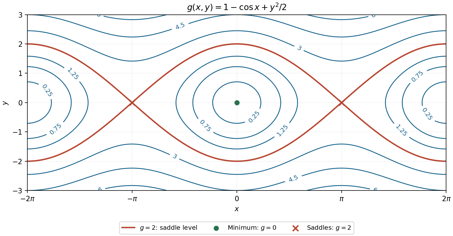
Contours of the cosine-plus-quadratic function, with its saddle level and stationary points labelled
. Details. 
Articles by others on the same topic
There are currently no matching articles.