Group the polynomial into two pairs, then use the difference of two squares:Thus is a double polynomial root and is a simple polynomial root.
The repeated factor requires both a simple-pole and a double-pole term in the partial fraction decomposition. WriteMultiplying through gives . Substituting and gives and ; the quadratic coefficient then gives . Therefore
At a single point of contact the line is a tangent line, so its slope equals the derivative of the exponential function. At the contact coordinate ,Since , dividing gives , hence . To verify uniqueness, the difference has positive second derivative everywhere and its unique minimum is zero at . Thus this line touches the curve once.
Using the contact coordinate and substituting into the exponential function givesBoth the curve and the line with the slope found in part (a) pass through this point.
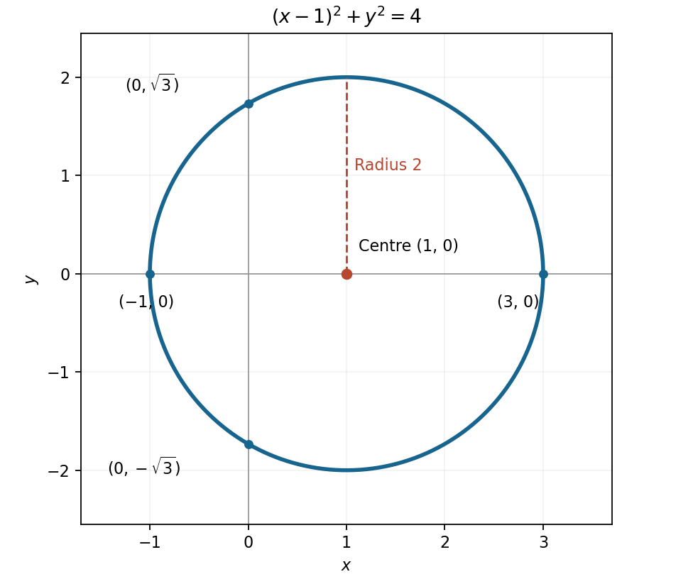
Use completing the square to obtainThe locus is therefore a circle with centre and radius . It meets the horizontal axis at and and the vertical axis at ; its highest and lowest points are .
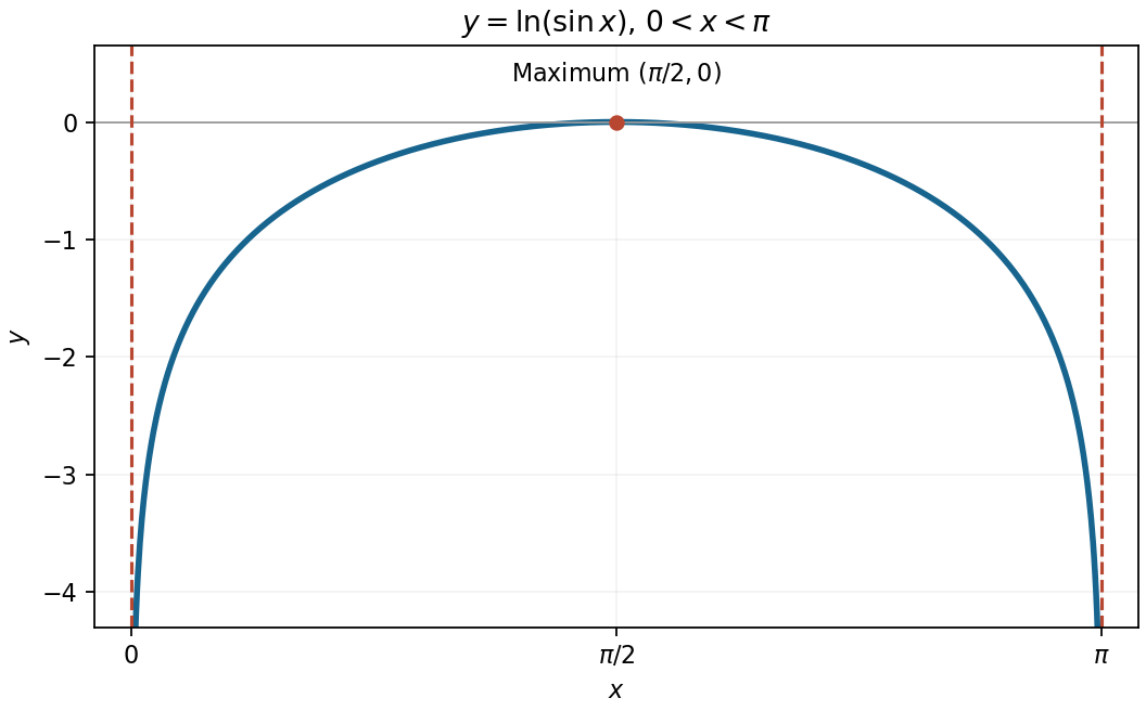
On any interval where , the chain rule gives . Differentiating again,The domain condition is necessary because the real natural logarithm requires a positive argument.
Within the requested interval, the function is symmetric about because . Its derivative is positive before , zero there, and negative afterwards. The negative second derivative shows that this is a strictly concave function. Consequently its unique maximum is . It tends to at both ends, giving vertical asymptotes and .
For the indefinite integral, substitute , so . An integration by parts then givesFor the definite integral, the original PDF's upper limit is , so the corresponding upper value of is . ThereforeBoth requested integrals are thus evaluated with the same antiderivative.
The maximum of sine is one. The allowed parameter values giving areSubstituting each into givesAll three parameter values lie in the original interval, so none of these maxima is discarded.
For this parametric curve, the chain rule givesThe quotient is a finite slope when . At and , the horizontal component of the tangent vanishes while the vertical component does not; these have vertical tangent lines, rather than missing finite values of the displayed quotient.
The usual interior condition for the binomial series is , giving as its open interval of convergence. In this particular square-root case the full series also converges absolutely at both endpoints, so the maximal real range on which its sum equals the original function isFor an endpoint check, write , where and . Then by telescoping, establishing absolute convergence at . The square-root binomial series at its endpoints proves continuity of the sum there. The endpoint values are at and at . Outside this range the power-series terms do not tend to zero. A three-term truncation remains an approximation, rather than an exact formula throughout the interval.
On the specified domain , so multiplying by is legitimate. Use the double-angle identity to findThe first factor gives . The second gives , yielding four more values in the interval. ThusEvery listed value has nonzero sine and satisfies the original equation. Dividing by would incorrectly lose the two solutions .
The positive horizontal coordinate is . By implicit differentiation,At the selected point this gives .
The normal line to a plane curve is perpendicular to the tangent line, so its slope is the negative reciprocal . The required equation isThe normal direction also agrees with the gradient of the defining level function.
The finite geometric series has eleven terms, from through . With common ratio ,Counting the powers explicitly avoids omitting the final term.
Direct substitution in the Möbius transformation givesNeither substitution meets the excluded denominator point .
For real , the numerator and denominator have equal complex modulus:The denominator is always nonzero. HenceThus the real axis maps into the unit circle in the complex plane.
Differentiate the polar form of a complex number using the product rule and chain rule:A second differentiation givesThe two contributions to arise separately from differentiating and from differentiating the moving exponential factor.
Write . Squaring the nonnegative complex modulus on each side givesThe linear terms cancel, leaving . Therefore the locus isIts real and imaginary axis intersections are and .
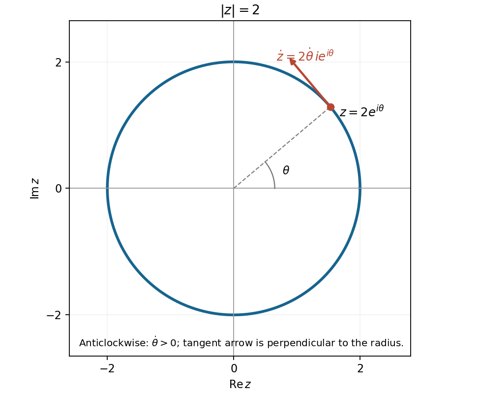
On this circle the radial coordinate is constant, , so . The velocity is a tangent vector to the circle in the anticlockwise direction, represented by when . Substituting into part (b),The inward component is the centripetal acceleration; the transverse component allows the speed to change. Anticlockwise motion does not imply uniform speed or . The preceding figure includes the required tangent arrow.
The perpendicular unit vectors represented by and point radially outwards and transversely in the increasing-angle direction. Reading off their real coefficients in part (b) gives the signed componentsThese are velocity in polar coordinates and acceleration in polar coordinates. In particular is a transverse speed component; alone is an angular velocity. The moving basis, rather than any extra force assumption, accounts for the additional acceleration terms. At the origin the polar directions themselves are undefined, although the Cartesian velocity and acceleration can remain well defined.
The two coefficients are the corresponding partial derivatives of . Therefore the differential form is exact, withThe arbitrary constant does not change the total differential.
For a smooth exact differential form , its coefficients must satisfy by Clairaut's theorem. HereThese are not equal as functions on the plane, so the form is not exact. Equality at isolated points or along some lines is insufficient: an exactness test must hold throughout an open domain.
The coefficients follow by differentiating the same monomial:Thus this exact differential form hasExhibiting a global scalar potential proves exactness directly, without needing an additional domain argument.
The partial derivatives are and , so all stationary points are for integers . Their Hessian matrix is . At even multiples of it is a positive-definite matrix, whereas at odd multiples it has one positive and one negative eigenvalue. ConsequentlyThere are no local maxima. Since both and are nonnegative, these are also global minima. In the requested open plotting window, the stationary points are and ; the local minima at lie on excluded edges.
For a level set , solving for the vertical coordinate givesFor these level sets are closed ovals around each local minimum. At the level sets shrink to the local minima. The level set through the saddle points iswhere the two signed branches together describe the same set as . They cross at and reach . The crossing slopes at a saddle point are , as also follows from the local quadratic form . For , the upper and lower level sets remain separate and extend across the plotting window without meeting the horizontal axis.
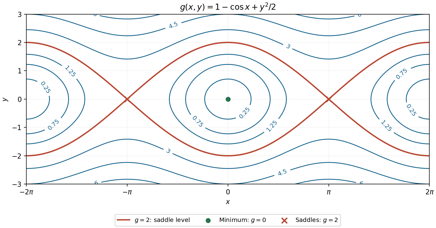
Contours of the cosine-plus-quadratic function, with its saddle level and stationary points labelled
. Details. Set . The similarity solution uses , whose partial derivatives at fixed or areApply the multivariable chain rule to :Substituting in the heat equation and cancelling the positive common factor gives
For a Gaussian function, the required derivatives areSubstitute these into the reduced ordinary differential equation and compare the constant and quadratic coefficients:The constant terms give , and this value also satisfies the quadratic terms. HenceA constant multiple is also a solution by linearity.
The heat equation is linear and homogeneous in : the operator satisfies . Thus the superposition principle applies to its solutions. Spatial translations are also allowed because the coefficients are constant.
Choose in part (b) and multiply by to make the initial amplitude one. Taking the two shifts and then givesAt this reproduces both initial peaks. Each term is an instance of Gaussian initial data for the heat equation, so their sum satisfies the equation. Its extension to negative times is a real smooth solution precisely on the connected intervalAt the lower endpoint the peaks narrow without bound and their heights diverge; there is no finite classical continuation there. For positive times each peak spreads and decreases in height while preserving its integral.
Differentiate the cycloid parametrization:The half-angle simplification is valid throughout , where . In particular the horizontal coordinate increases strictly along the arch.
The cycloid has limiting endpoints and , with its highest point at . The transformation sends to and preserves , so the arch is symmetric about . Its slope decreases from through zero to , giving vertical limiting tangent lines at the cusps and a horizontal tangent line at the top. More explicitly,so the arch is a concave function throughout its interior. The endpoint cusps are limiting points, excluded by the open parameter interval.
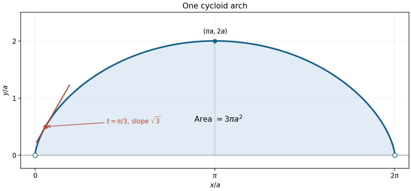


The original PDF specifies slope ; the transcription's is erroneous. By part (a), . Since and cotangent is strictly decreasing there, the unique parameter value is . ThereforeThe tangent line drawn in the preceding figure has the required positive slope.
Because along the arch, its area above the baseline is the definite integral . Changing to the parameter givesAdding or removing the two endpoint points does not change the area. This is the area formula in area and length of a cycloid arch.
The arc length follows from the speed of the parametrization:Here inside the given interval. ThereforeThe result scales as a length, while the preceding area scales as , as required by dimensional analysis.
For , Taylor's theorem after terms, counting the constant term, isUnder the usual hypothesis that is times continuously differentiable on the interval joining and , and times differentiable in its interior, the Taylor theorem with Lagrange remainder givesThis is a finite expansion with a controlled remainder; it does not assume an infinite Taylor series converges. For the remainder is zero.
Let near . The chain rule givesSubstitute into the first three terms of the Taylor expansion:The quadratic coefficient is , not . The apparent square root creates no local difficulty at the positive expansion point.
Use the Maclaurin series and . Multiplying through the cubic order givesThese are the first three nonzero terms; the constant term vanishes.
Both numerator and denominator vanish quadratically. Factor out before dividing the power series:The reciprocal of the denominator is . HenceThe expansion describes the continuous extension at the removable singularity , where the original quotient is undefined but its limit is one. Odd powers vanish because the quotient is even.
Uniform sampling without replacement is equivalent to revealing a uniformly random permutation of seven labelled balls. Each draw position is equally likely to contain any label, so its colour has the original proportions. ThusFor example the law of total probability gives . Equal marginal probabilities express exchangeability, rather than independence between successive draws.
The first black draw has probability . Given that event, three of the remaining six balls are black. The multiplication rule therefore givesUsing would incorrectly treat the draws as independent.
Articles were limited to the first 100 out of 151 total.
Articles by others on the same topic
There are currently no matching articles.